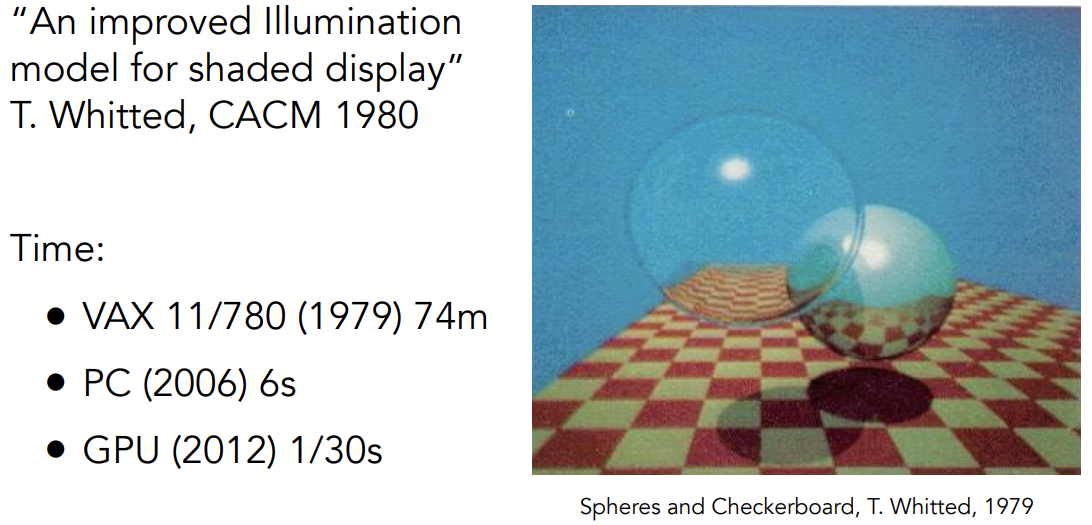
Games101课程笔记(二)
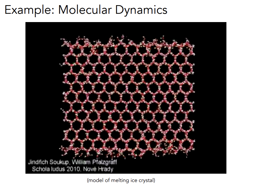
光线追踪 Ray Tracing
Why Ray Tracing
-
光栅化不易于把一些全局的效果处理好
-
阴影(软阴影)
-
尤其是光线的多次反射(Glossy reflection, indirect illumination)
-
-
光栅化很快,但是质量相对较低(一种快速的近似)
-
光线追踪很准确,但是很慢
- Rasteriaztion:real-time,Ray Tracing:offline
- 生成1帧图大概需要渲染10k CPU hours
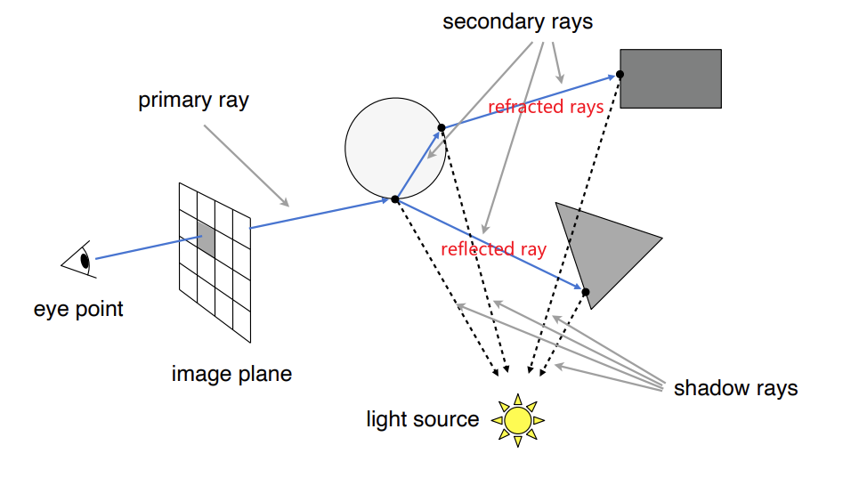
Basic Ray-Tracing Algorithm
Light Rays
关于光线的三个idea:
- 光沿直线传播(虽然实际上是错的)
- 即使光线之间彼此相交,光线也不会与彼此发生碰撞
- 光线从光源沿着一定的路径射向眼睛,且光路可逆
实际上光线追踪是从相机出发向世界中投射光线
Ray Casting
光线投射
-
从相机处此处认为相机是一个点),对成像平面上的每一个像素向场景中投射光线,记录最近的交点(类似深度)
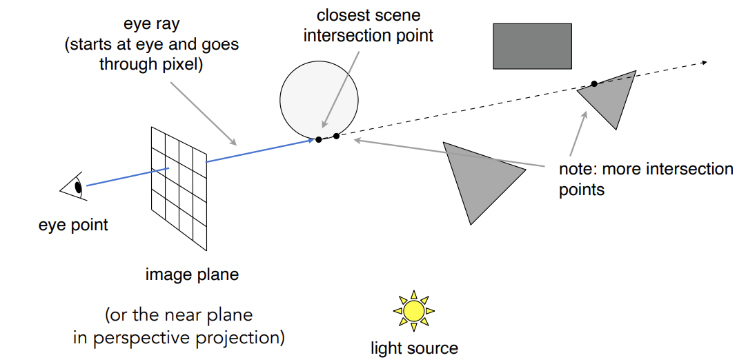
-
(考虑记录的交点会不会被照亮)连接交点和光源(shadow ray),如果shadow ray上没有其他物体,那么说明这个交点被光源照亮,再执行shading计算得出像素的颜色
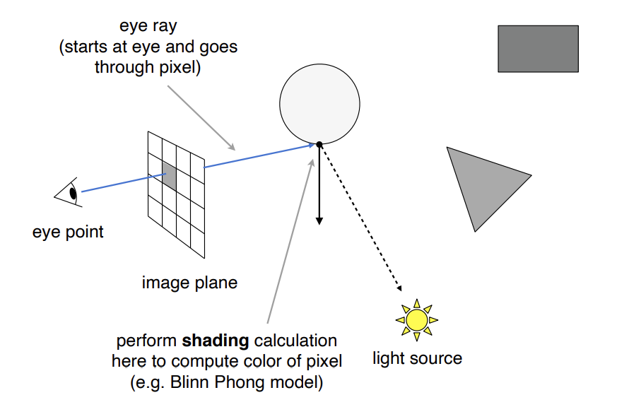
局限:还是只考虑了一次光线的反射
Recursive(Whitted-Style) Ray Tracing
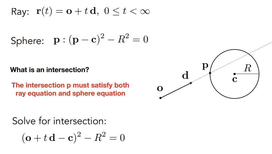
Ray-Surface Intersection
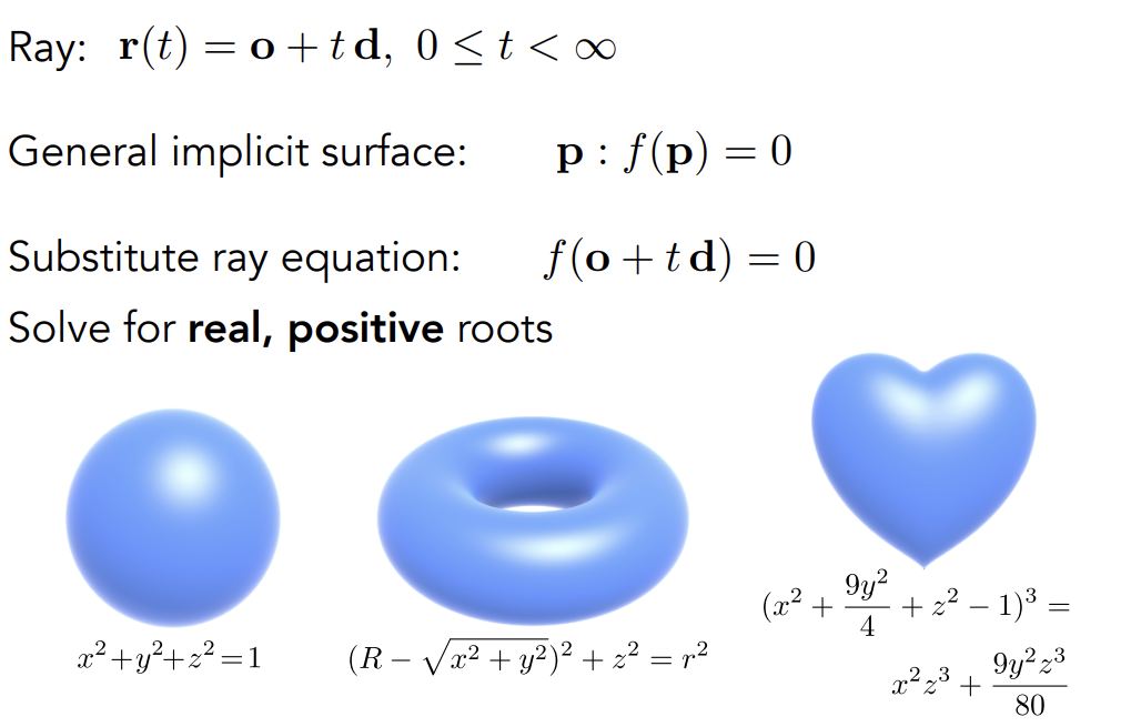
Ray Equation
- 用==光源==和==一条方向向量==定义光线
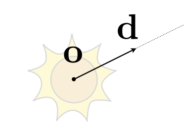
- Ray Equation:( :时间,非负 )
- Ray Intersection with Sphere:
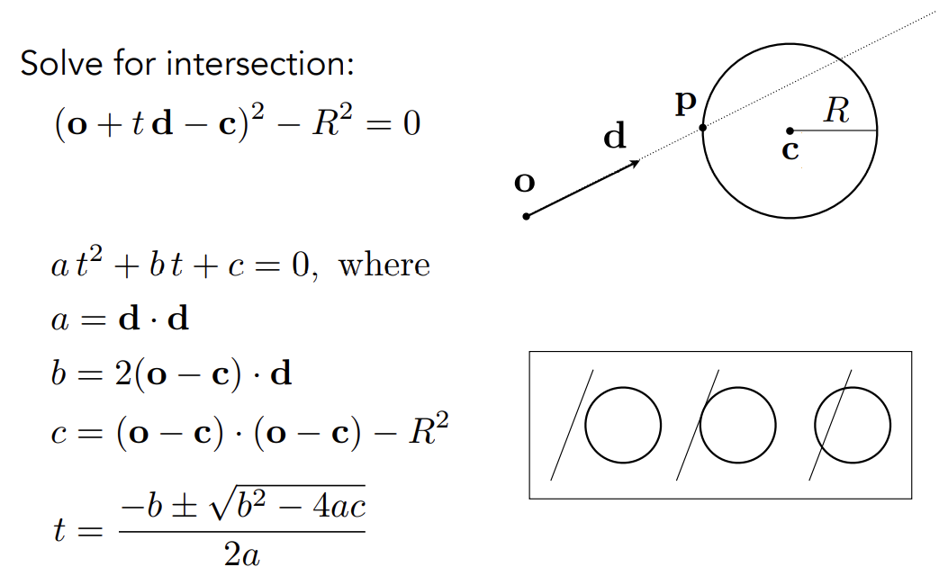
- 推广到光线与Implicit Surface隐式表面的求交:
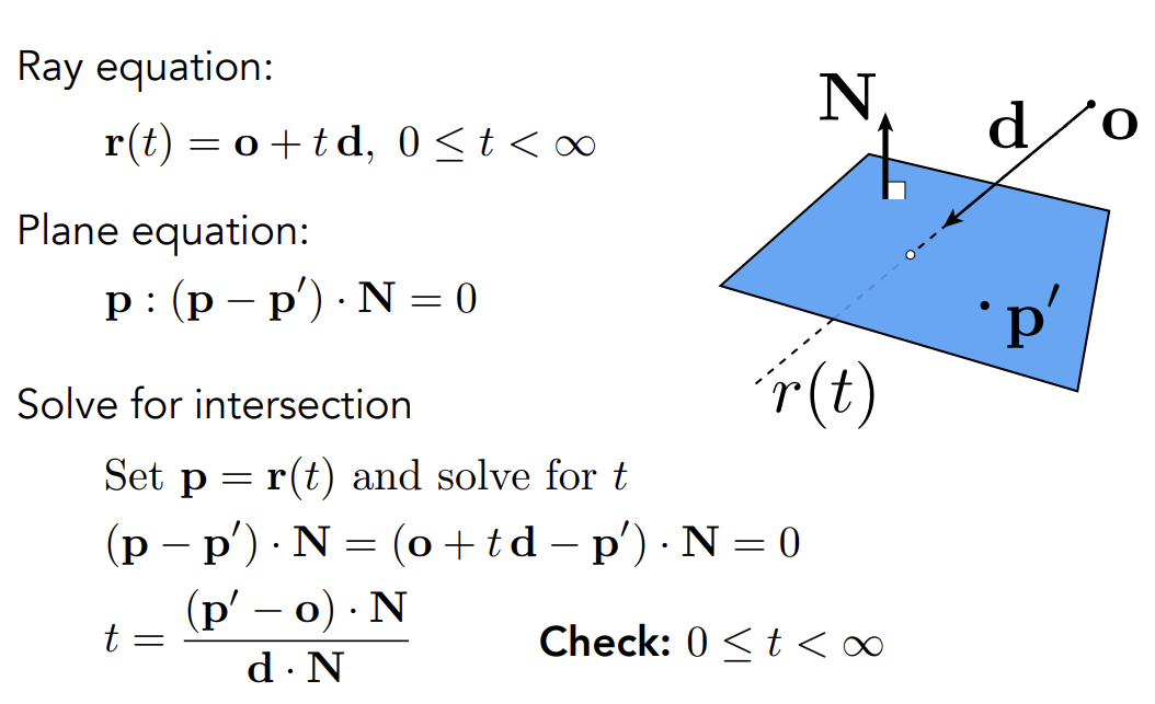
Plane Equation
- 用==一个点==和==一条法线向量==定义一个平面
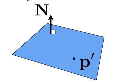
- Plane Equation:
-
光线和三角形面求交:
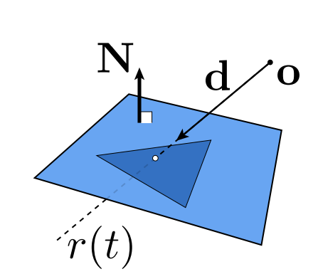
转换为两步:
-
光线与平面求交
-
然后再通过cross判断交点是否在三角形内部即可
-
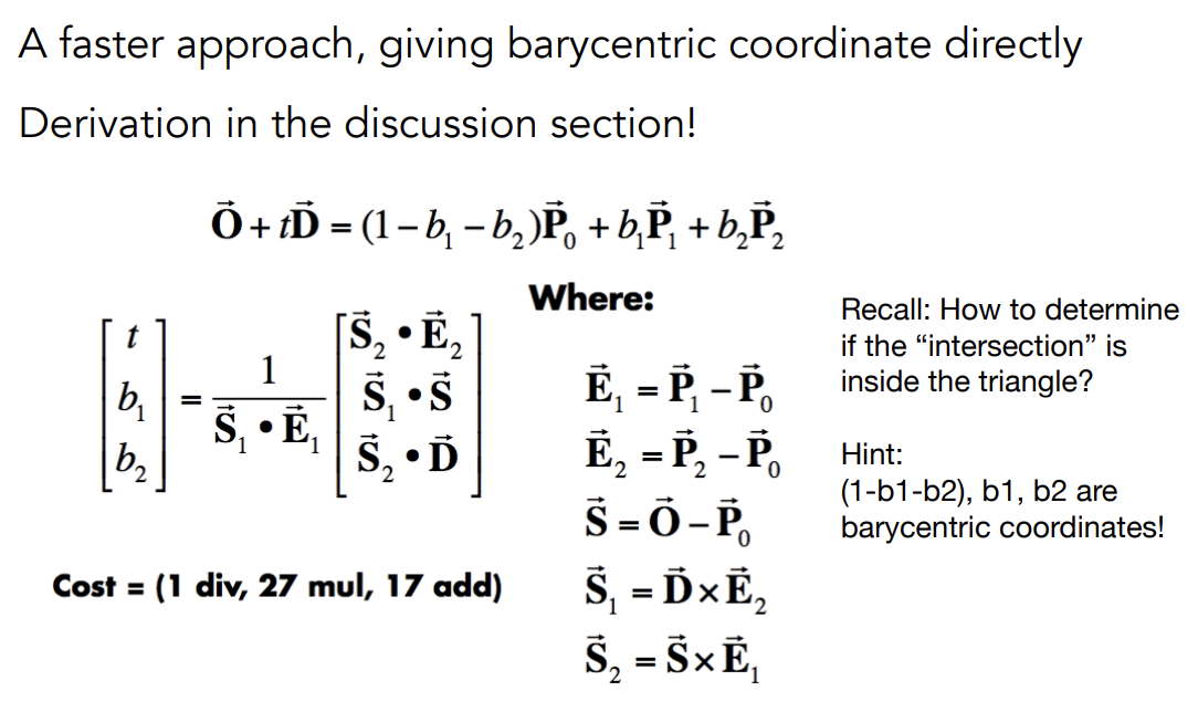
Moller Trumbore Algorithm
简化三角形和光线求交的算法
原理:一个点在三角形内,那么就可以写为重心坐标的形式,那么一个交点就应该同时满足光线方程和存在三角形重心坐标两个条件(通过三者之和等于一和及三者非负即可判断点在三角形内)
Accelerating Ray-Surface Intersection
Bounding Volumes(BVol)
- 一个可以完全包围物体的体积
- 如果光线不hit包围盒,他就不会hit物体
- 所以可以先检测BVol是否被hit,如果hit了再检测物体

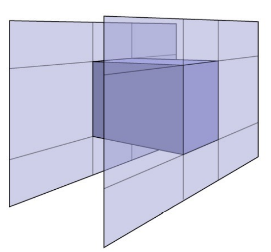
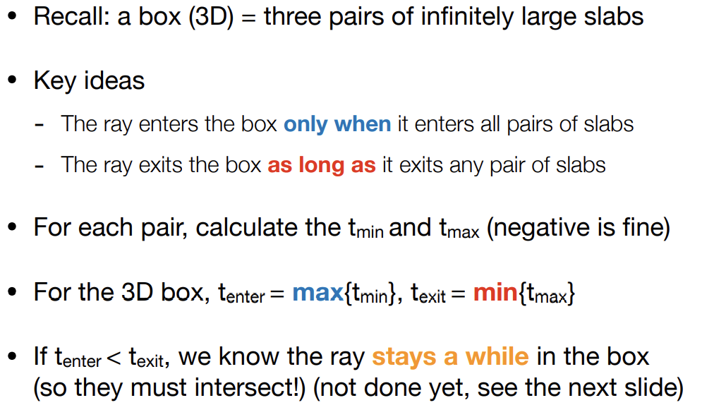
Ray-Intersection with Box
理解Box:Box是三组相对的面形成的交集(Box is the intersection of 3 pairs of slabs)
通常用Axis-Aligned Bounding Box(AABB)(轴对齐包围盒)
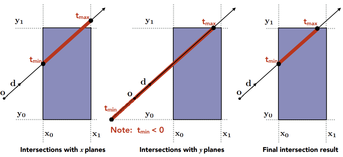
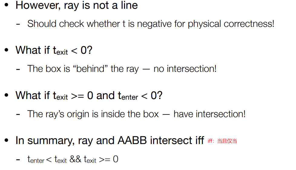
Ray Intersection with Axis-Aligned Box
原理:计算光线和平面相交的时间,并判断得到光线在BVol内部的时间(起始时间为最后一个轴向的进入时间,结束时间为最早一个轴向的离开时间)
三维空间中:
为什么用Axis-Aligned的绑定盒:极大地简化加速求交
用随意的包围盒,进行求交时要做三个轴向上的减法,再乘法线,就会有3次减法,六次乘法和一次除法
而用轴向包围盒,只需要考虑一个轴向的距离,除上光线在该轴的分量即可
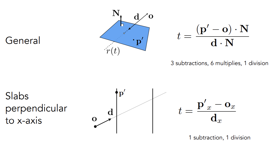
AABB totally : 3 subtraction, 3 division, get min and max
Using AABBs to accelerate ray tracing
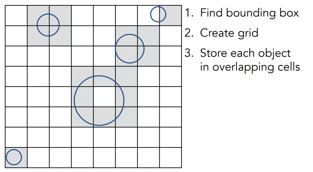
Uniform Spatial Partition(Grids)
Preprocess — Build Acceleration Grid
找到场景的包围盒,在包围盒内划分网格,判定哪些网格里与物体相交并标记与物体相交的网格(只考虑表面不考虑内部)
Ray-Scene Intersection
投射光线,顺着光线方向与一个一个的盒子求交,对于预处理过程中没有被标记的盒子不需要做与实际物体求交的操作;当光线遇到在预处理过程中被标记的盒子时,意味着这个盒子里会有物体,光线有可能会与物体有交点,所以需要在这个格子内与物体求交进行判断;当找到光线与物体的第一个交点后光线就可以停下来了
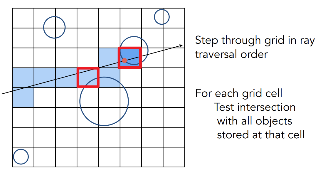
”沿着光线方向“的实现方法:(一种没有在用但是很好理解的方法)光栅化一条直线的方法:知道这个盒子现在在和光线求交,那么下一次和光线进行求交的一定是他周围的盒子
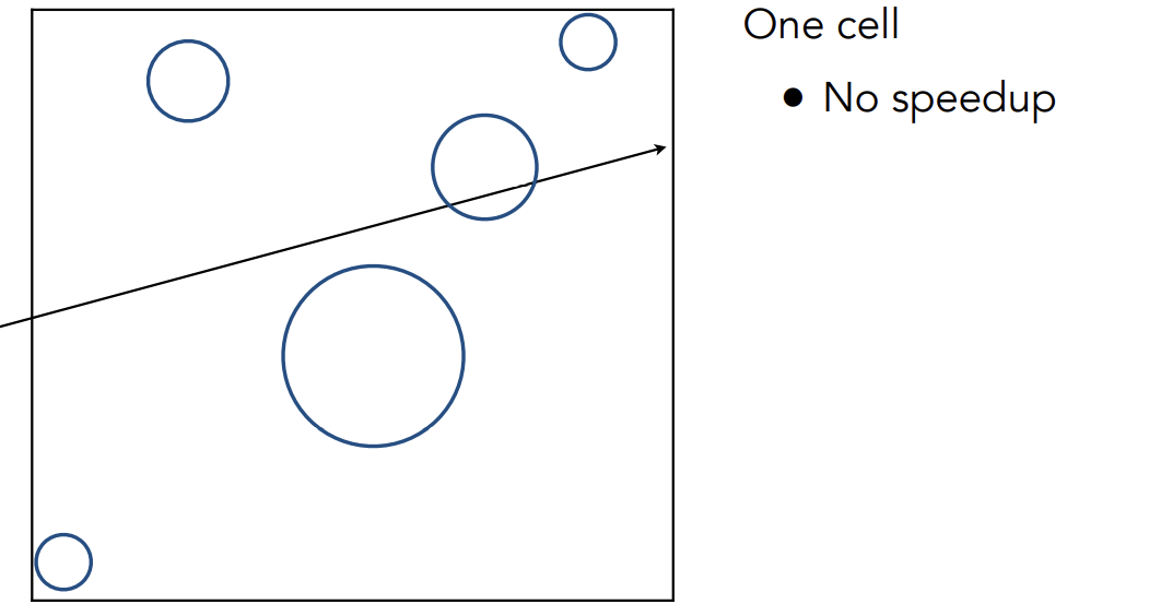
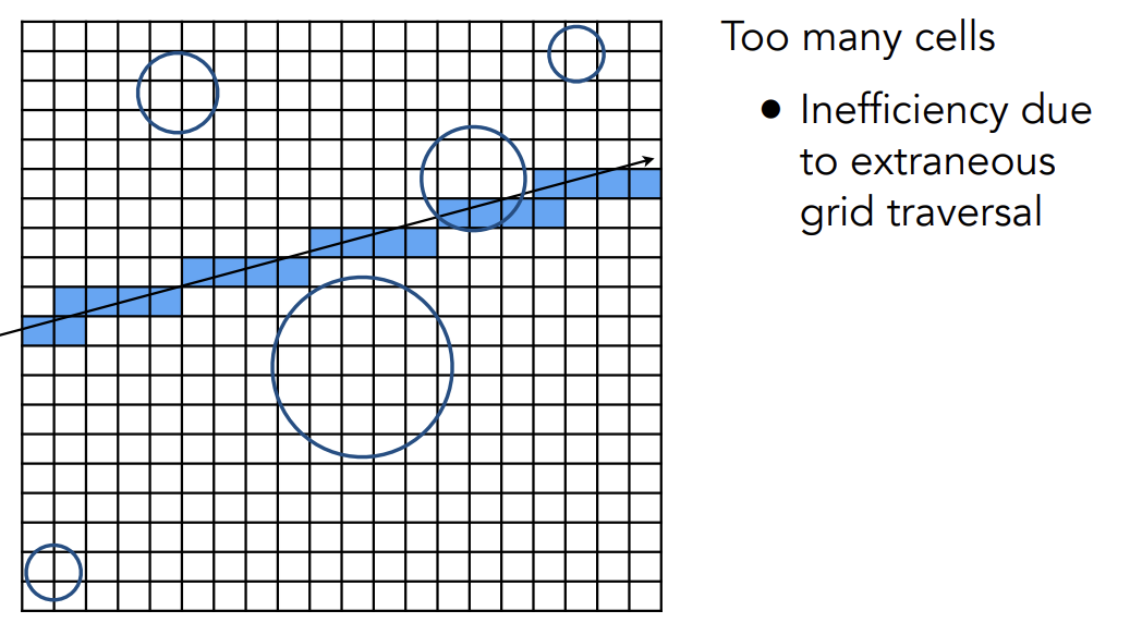
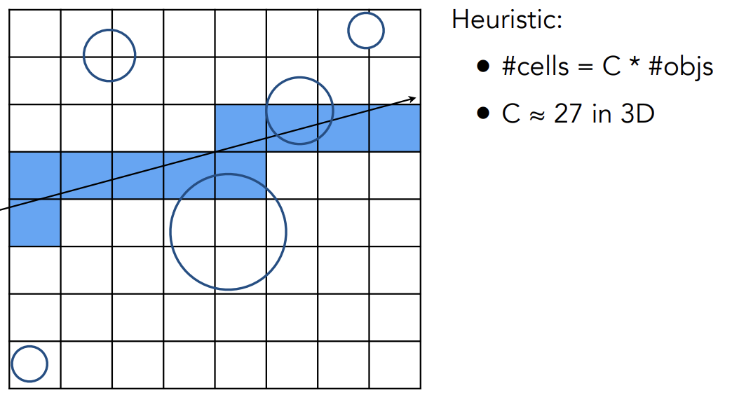
Grid Resolution
包围盒内的网格太密集太疏松都不好
效果不错的格子数量:(这也并非游戏中实际使用的方法,因为它还是要走过他所相交的所有格子,只用知道Grid数量不能太多或太少,有一个平衡就好)
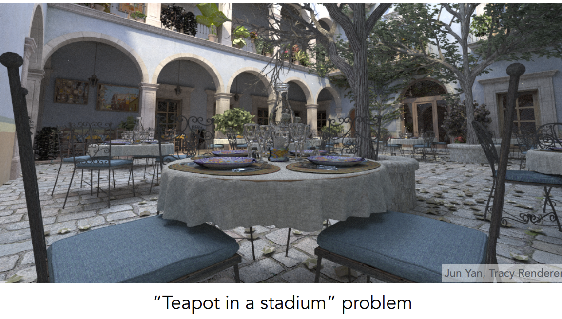
When Uniform Grids Fail
适合应用于场景中有很多物体的情况
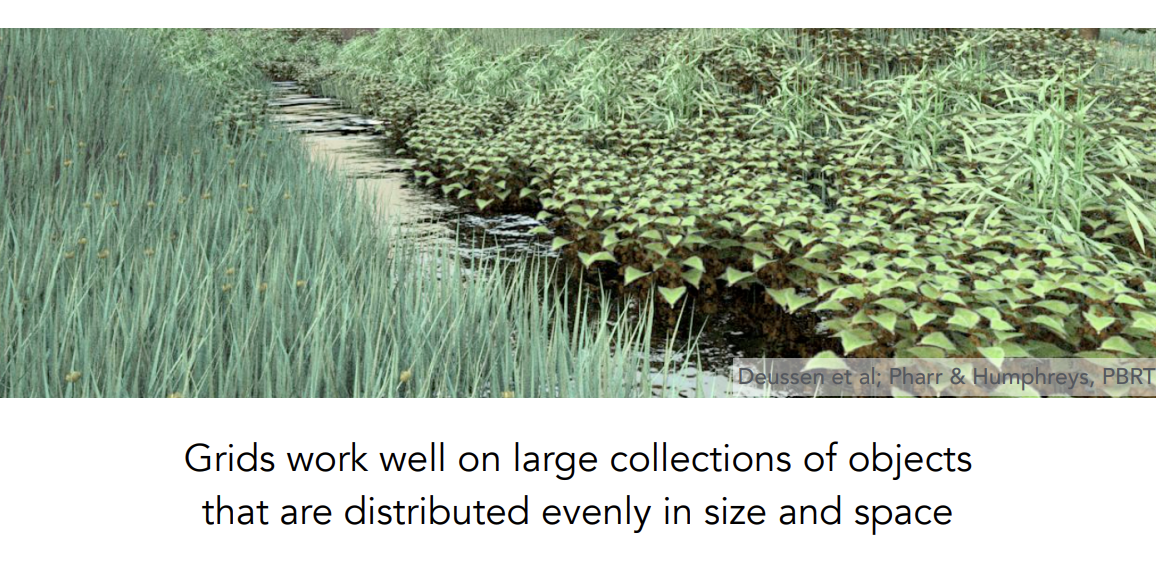
但是不适合用于场景很空的情况——”Teapot in a stadium“ problem
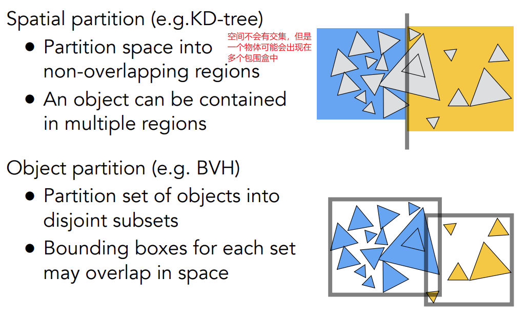
Spatial Partitions
Spatial Partitioning Examples
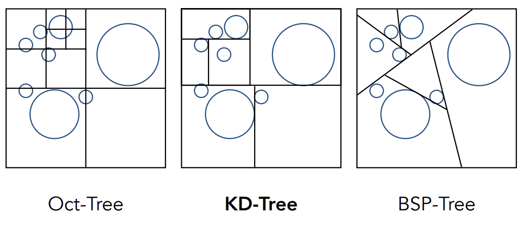
- Oct-Tree:八叉树(平面情况是四叉树——和维度绑定,在高维度不好计算)
- KD-Tree:和八叉树几乎完全相同,区别在每次找到一个物体就会在轴向上砍一刀,形成类似二叉树的结构;KD-Tree是层之间循环轴向切割,即这一层沿着x方向,下一层就沿着y方向,再下一层沿着z方向,以xyz顺序循环
- BSP-Tree:每一次选一个方向将节点砍开,与KD-Tree区别在于不是横平竖直地砍,且在高维度会不好计算
KD-Tree Pre-Processing
在进行光追前先做好加速结构,再去考虑与光线求交
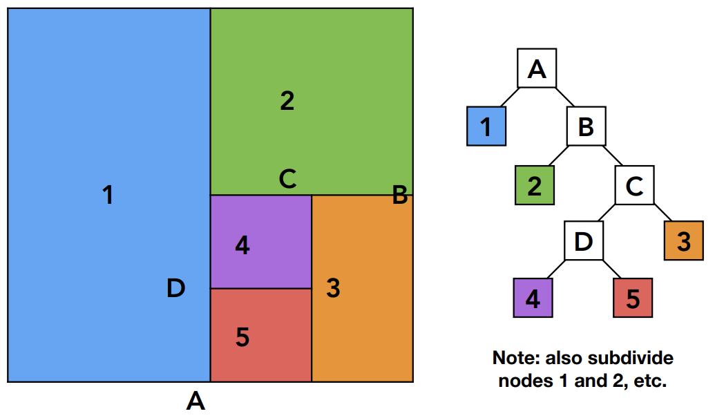
注:蓝色绿色部分都会砍开,只是没有画出来
- 中间节点只需要记录它会被如何划分
- 叶子节点(决定不再划分地节点)才需要再去存储和格子相交的几何形体的信息
Data Structure for KD-Trees
中间节点存储:
- 该节点向下分裂的轴向
- 平面沿着轴向的分裂位置
- 指向子节点的指针
- 实际物体不会储存在中间节点内
叶子节点:
- 储存实际物体的链表
Traversing a KD-Tree
光线照射进入BVol
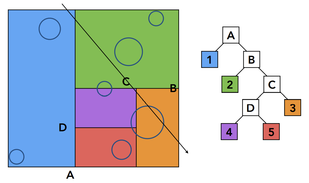
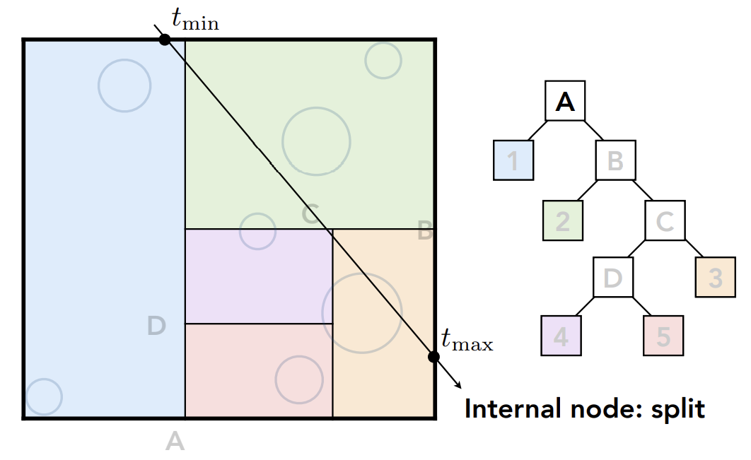
发现A内有物体,就需要和A的两个子节点都进行求交(A有分支,就对A和他的子分支求交,以此递归,直到找到叶子节点)
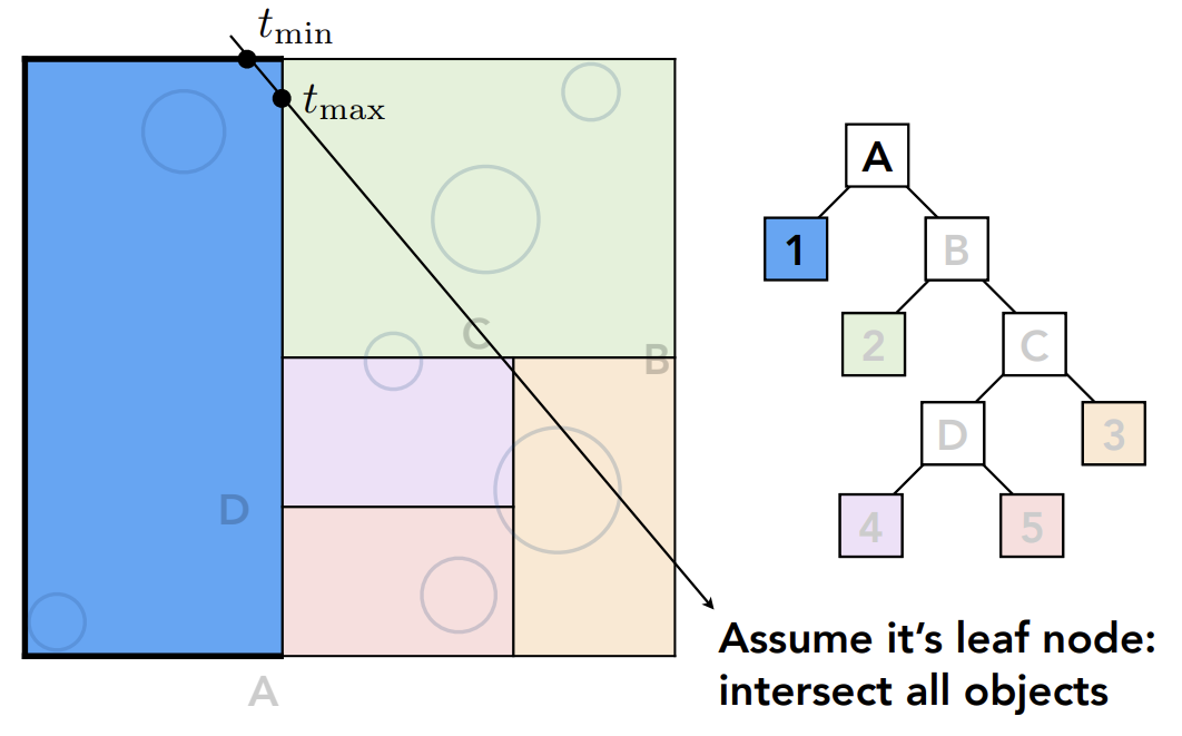
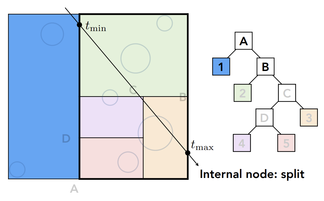
以此向下进行
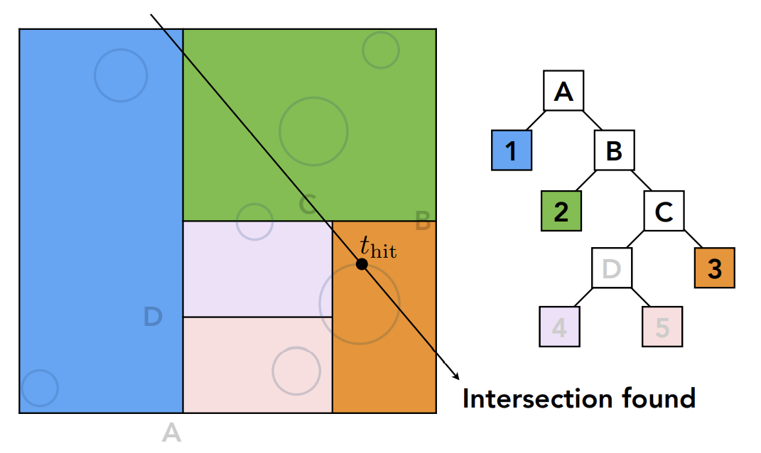
即:光线如果和该节点有交点,那么光线会向下对该节点的两个子节点求交;如果光线和该节点没有交点就不会继续对该节点的子节点求交;以此向下进行,直到找到叶子节点
Problem
- KD-Tree的建立不简单,需要考虑三角形与盒子的求交(举例:三角形三个顶点不在盒子内,但是这个盒子内有三角形的一部分的情况,不容易处理三角形与盒子的求交)
- 物体可能存在于多个盒子内
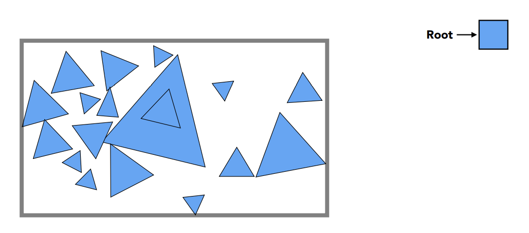
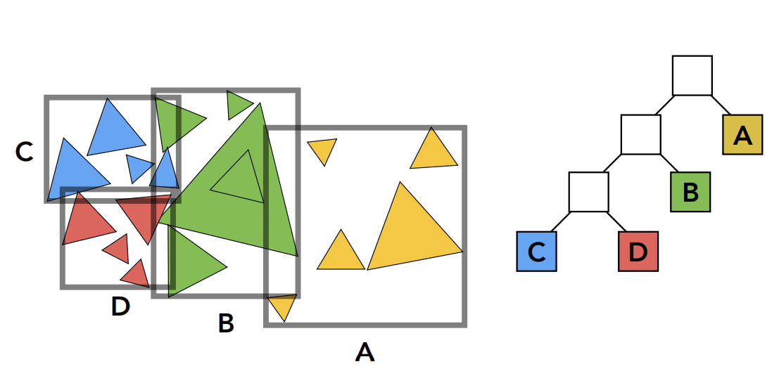
Object Partition & Bounding Volume Hierarchy(BVH)
以物体为根基,把物体”分堆“并重新计算他们的包围盒——解决了物体可能存在于多个盒子内的问题
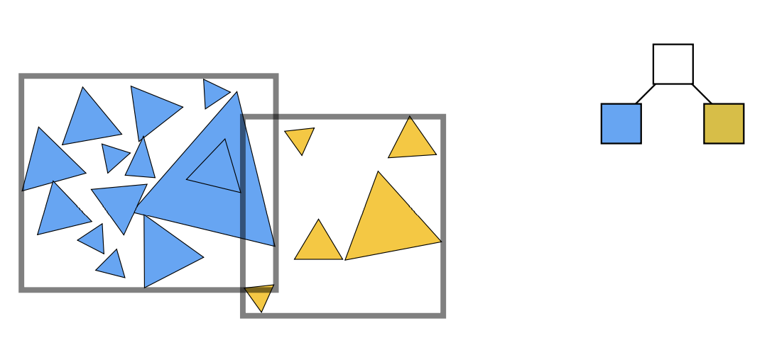
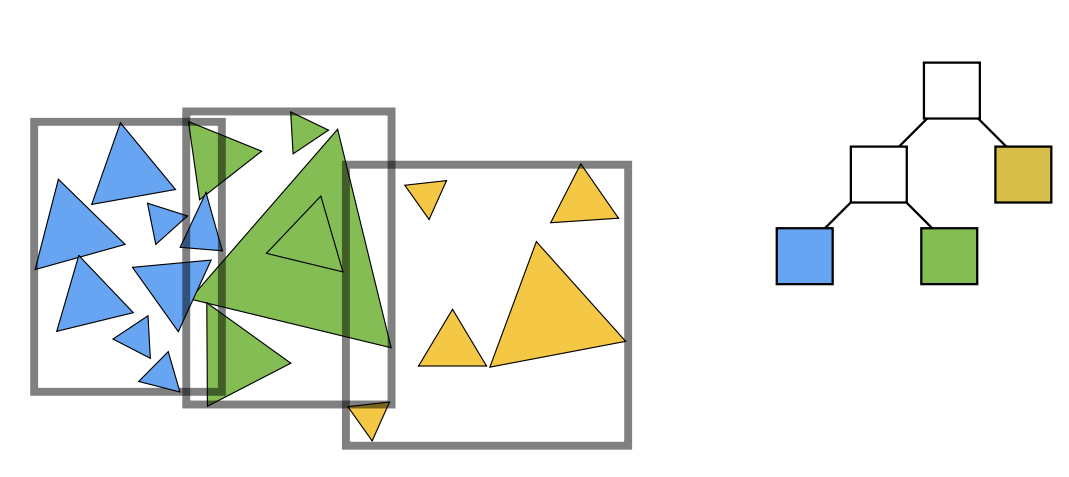
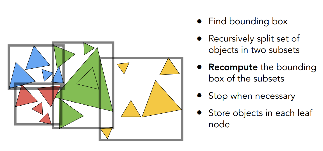
实际上如何划分一个节点:
- 选择一个维度去划分
- Heuristic ##1:总是沿着最长的轴去划分,让最长的轴变短,让整个结构最后变得均匀
- Heuristic ##2:取中间的物体进行划分(第个),让这棵树接近平衡
- 无序的一列数快速找出中位数(不需要排序):快速选择算法,只对快排划分出的某一边进行操作,可以使时间复杂度在以内
最终取值:
- Heuristic:节点内含有少量元素时终止
Data Structure for BVHs
中间节点存储:
- 包围盒
- 指向子节点的指针
叶子节点存储:
- 包围盒
- 存储实际对象的链表
节点代表场景中原始物体的交集
- 所有物体都在subtree中
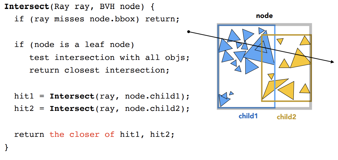
BVH Traveral
Spatial vs Object Partitions
Basic Radiometry
—— 辐射度量学
why radiomentry
Radiometry
-
Measurement system and units for illumination
-
精确测量光在空间中的属性,并且还是基于几何光学(光沿直线传播,不考虑波动性)
- New terms:Radiant flux,intensity,irradiance,radiance
-
辐射度量学实际上是在物理上准确定义光照的方法
Radiant Energy and Flux(Power)
######## Radiant Energy
Radiant energy是电磁辐射的能量,以焦耳为单位,用符号表示:
######## Radiant flux(power)
单位时间内发射、反射、转换或接收的能量
(lumen是光学上的单位,理解为光的亮度)
Flus —— 单位时间通过感光位置的光子量
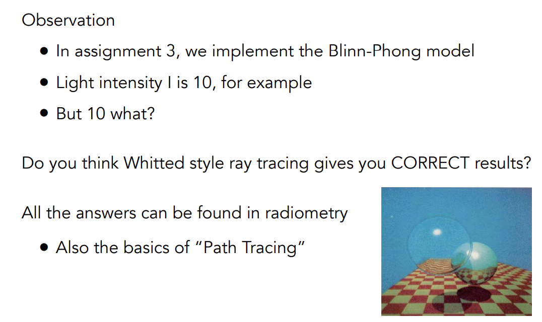
Radiant intensity
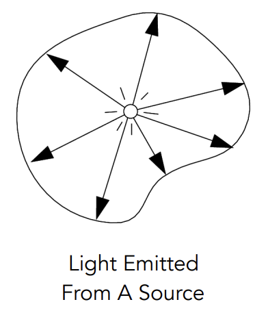
######## Definition
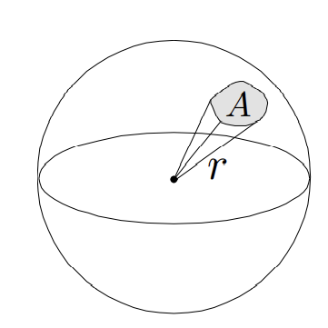
The radiant (luminous) intensity is the power per unit solid angle emitted by a point light source
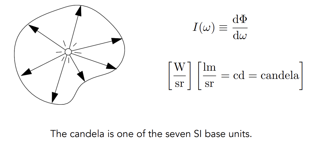
######## Solid angles and Solid angle
Angle: ratio of subtended arc length on circle to radius
-
-
Circle has 2 radians
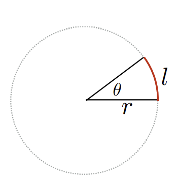
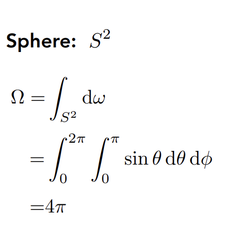
Solid angle: ratio of subtended area on sphere to radius squared
-
-
Spere has 4 steradians
-
弧度在球面上的延申——球弧度,立体角描述空间上的角张开的大小
######## Differential Solid Angles
微分立体角:理解为取一个方向在球面上打到的点,再将这个方向向量的和都增加一个极小的量,最后投影到球面上得到的一个小曲面对应的立体角
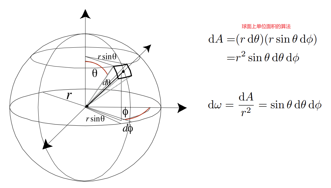
对微分立体角在整个球面上积分可以得到整个球的表面积
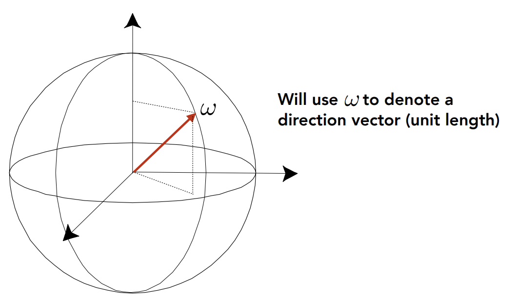
######## as a direction vector
######## Isotropic Point Source
Radiant intensity(intensity)就是单位时间内光源向各个方向发射的光子能量强度
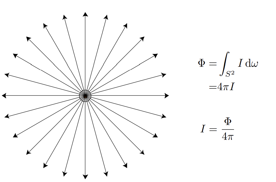
intensity是单位面积上的power,因此对intensity在面积上进行积分可以得到power
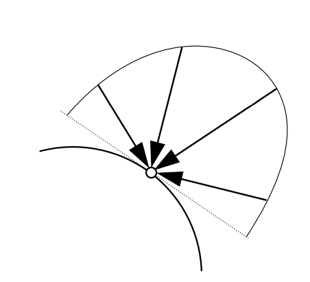
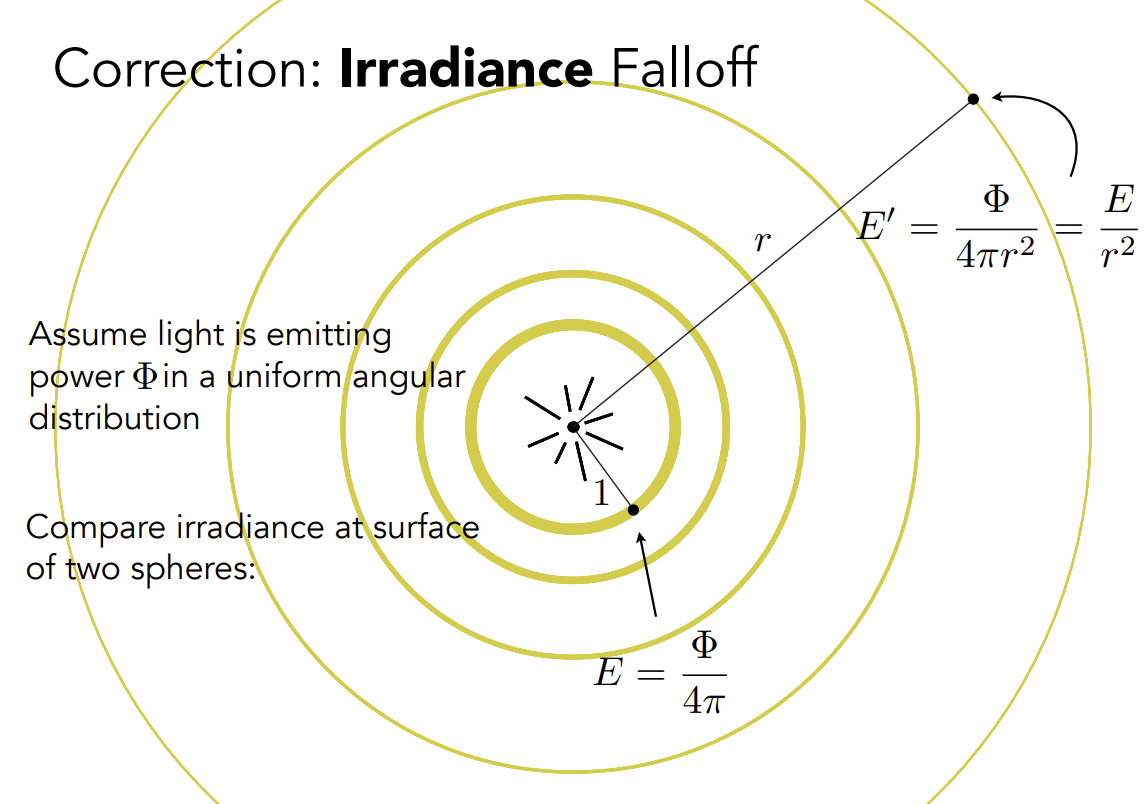
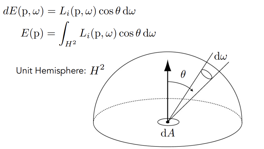
Irradiance
######## Definition
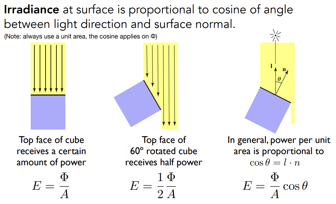
The irradiance is the power per unit area incident on a surfacec point
 $$
E_{(x)} = \frac{d\phi (x)}{dA}
\cr
[\frac{W}{m^2}][\frac{lm}{m^2}=lux]
$$
这个**area**必须是与光线垂直的部分,如果不垂直的话要把光线投影到垂直方向
$$
E_{(x)} = \frac{d\phi (x)}{dA}
\cr
[\frac{W}{m^2}][\frac{lm}{m^2}=lux]
$$
这个**area**必须是与光线垂直的部分,如果不垂直的话要把光线投影到垂直方向
- lambert计算漫反射时需要投影到垂直部分
-
四季的原因:
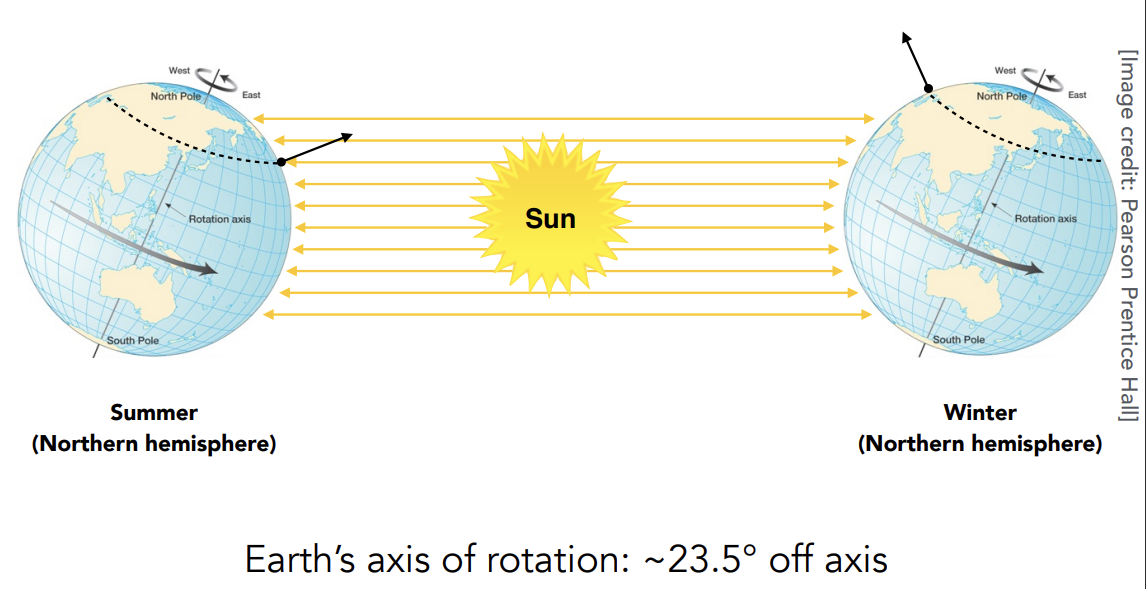
######## light Falloff
Light falloff的正确解释:不是intensity的衰减,而是irradiance的衰减,传播到越往外面积越小,irradiance越小
Radiance
######## Definition
The radiance (luminance) is the power emitted, reflected, transmitted or received by a surfae, per unit solid angle, per projected unit area
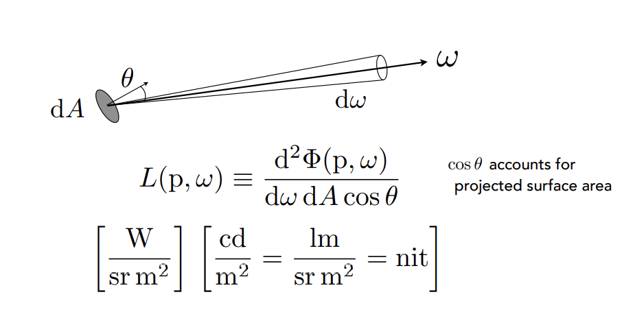
对power的两次微分:单位立体角、单位投影面积
一个单位面积可能和光的朝向不垂直,在度量特定方向的光的朝向时需要进行投影,即需要确定某一个特定的面和某一个特定的方向,通过这样的方式去定义光线
######## Radiance comprehension
Recall
- Irradiance:power per projected unit area
- Intensity:power per solid angel
So
- Radiance:Irradiance per solid angle
- Radiance:Intensity per projected unit area
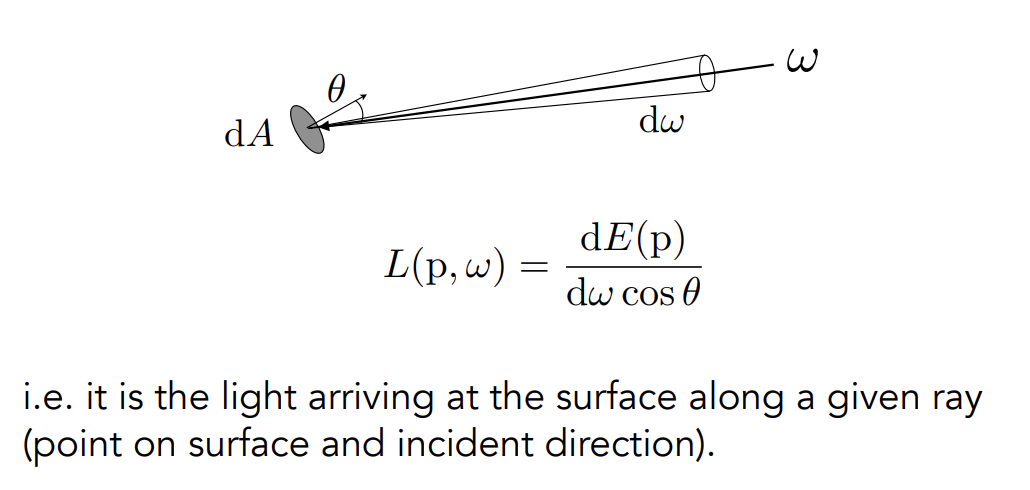
######## Incident Radiance
一个面接收到的能量:
入射Radiance是单位立体角上的到达入射表面的irradiance,即radiance和irradiance的区别在于是否有方向性
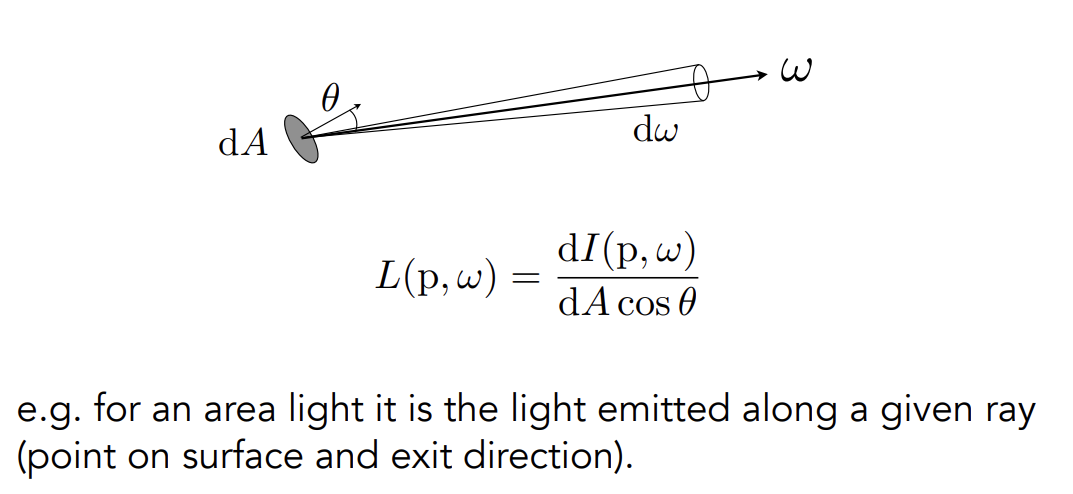
######## Exiting Radiance
一个面发射出去的能量:
出射Radiance是在单位投影面积上的intensity,即radiance和intensity的区别在于是否投影到单位面积
######## Irradiance vs. Radiance
Irradiance:一个很小的范围收到的所有的能量
Radiance:一个很小的范围收到的特定方向的能量
BRDF and Rendering Equation
Bidirectional Reflection Distribution Function 双向反射分布函数
BRDF
反射的解释:
Radiance从方向打到成为接收到的power,然后power会成为向任意的方向的Radiance
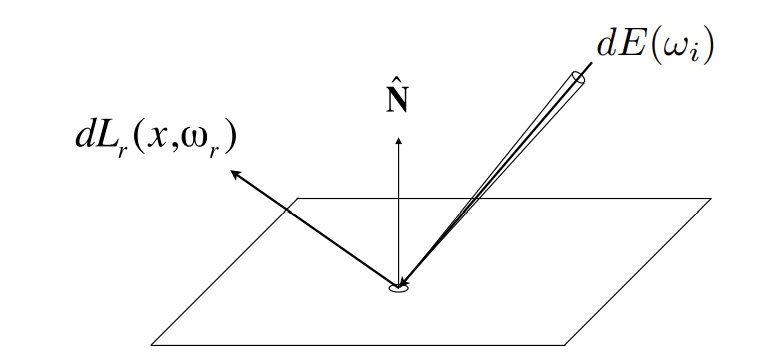
Differential irradiance incoming:
Differential radiance exiting (due to ):
BRDF的解释:
定义一个函数,描述微小面积,从某一个微小立体角接收到的irradiance会如何被分配到各个不同的立体角上去,即一个比例,任何一个出射方向的radiance去除以这一个小块接收到的irradiance
BRDF的定义:
The Bidirectional Reflection Distribution Function respresents how much light is reflected into each outgoing direction from each incoming direction
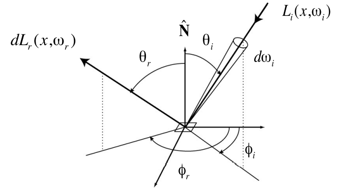 $$
f_r(\omega_i\rightarrow\omega_r)=\frac{dL_r(\omega_r)}{dE_i(\omega_i)}=\frac{dL_r(\omega_r)}{L_i(\omega_i)cos{\theta_i}d\omega_i}[\frac{1}{sr}]
$$
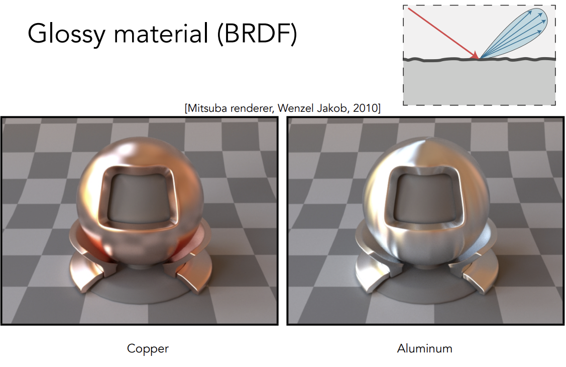
BRDF理解:从一个方向进来,打到物体后,物体向各个方向反射的能量分布情况。比如说物体是镜面的,镜面反射方向分分布了所有能量,其他方向没有能量;如果是漫反射,能量会均等的向各个方向分布。BRDF描述了光线和物体如何作用,他决定了物体不同的材质会怎么回事
$$
f_r(\omega_i\rightarrow\omega_r)=\frac{dL_r(\omega_r)}{dE_i(\omega_i)}=\frac{dL_r(\omega_r)}{L_i(\omega_i)cos{\theta_i}d\omega_i}[\frac{1}{sr}]
$$
BRDF理解:从一个方向进来,打到物体后,物体向各个方向反射的能量分布情况。比如说物体是镜面的,镜面反射方向分分布了所有能量,其他方向没有能量;如果是漫反射,能量会均等的向各个方向分布。BRDF描述了光线和物体如何作用,他决定了物体不同的材质会怎么回事
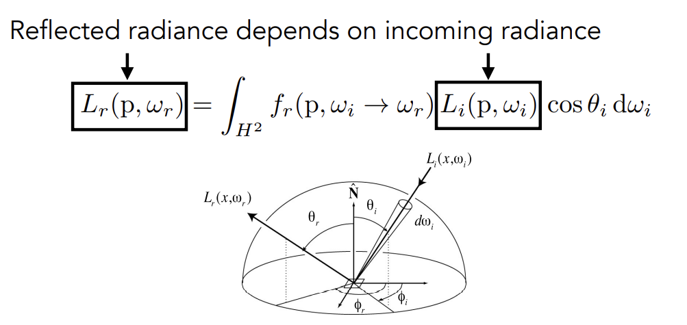
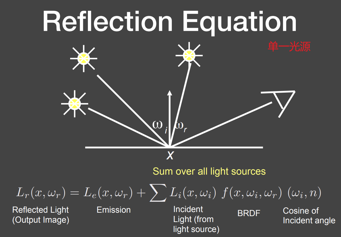
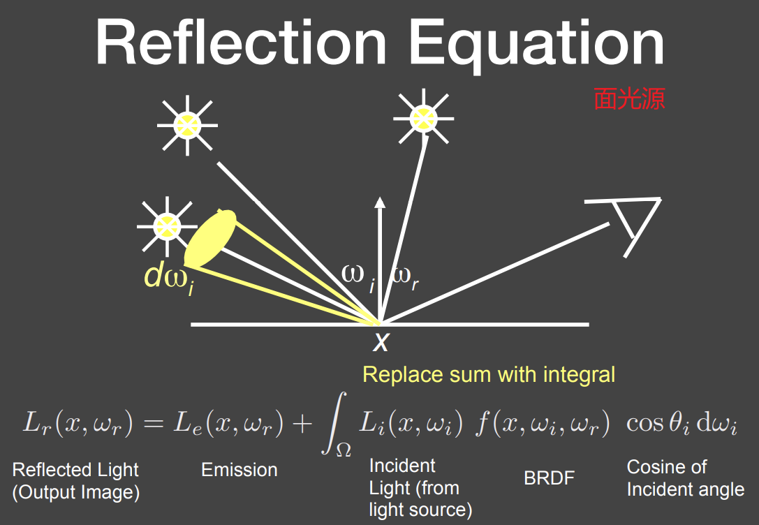
Reflection Equation
考虑入射的全部方向:反射方程
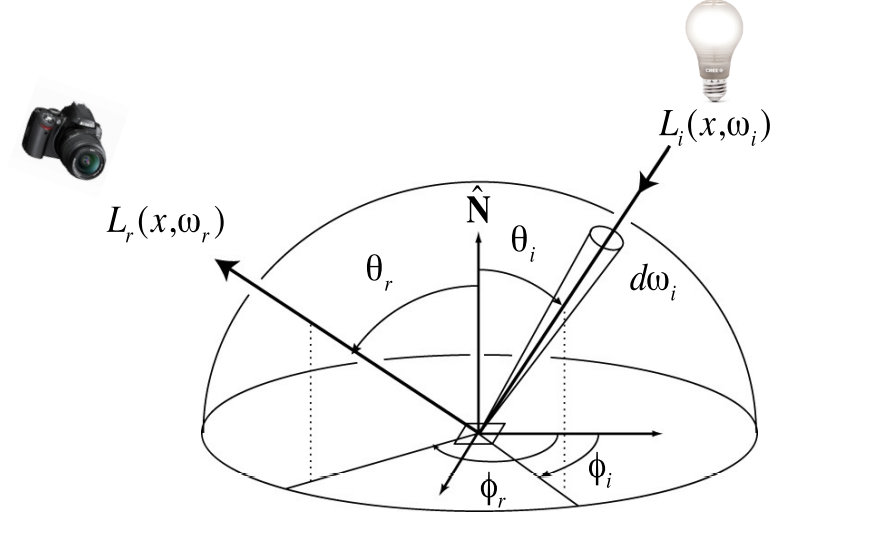 $$
L_r(p,\omega_r) = \int_{H^2}f_r(p,\omega_r \rightarrow\omega_r)L_i(p,\omega_i)L_i(p,\omega_i)cos{\theta_i}d\omega_i
$$
将所有入射方向的贡献积分起来形成最终的出射的radiance
$$
L_r(p,\omega_r) = \int_{H^2}f_r(p,\omega_r \rightarrow\omega_r)L_i(p,\omega_i)L_i(p,\omega_i)cos{\theta_i}d\omega_i
$$
将所有入射方向的贡献积分起来形成最终的出射的radiance
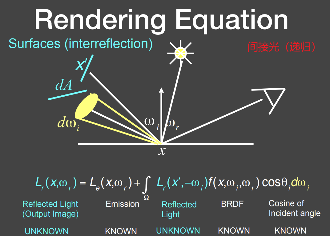
Challenge: Recursive Equation
光线在场景中不可能只弹射一次,任何出射的radiance都可能成为别的面的入射radiance,会存在一个递归的形式
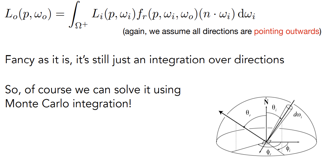
Rendering Equation
考虑自发光后:
- 假定所有方向都指向外
- 同都表示半球(下半球的光不会造成影响,所以考虑的只是半个球体,而非一个球体)
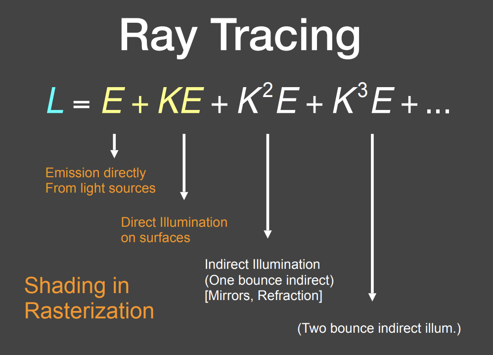
Summary
将渲染方程简化为一个积分方程
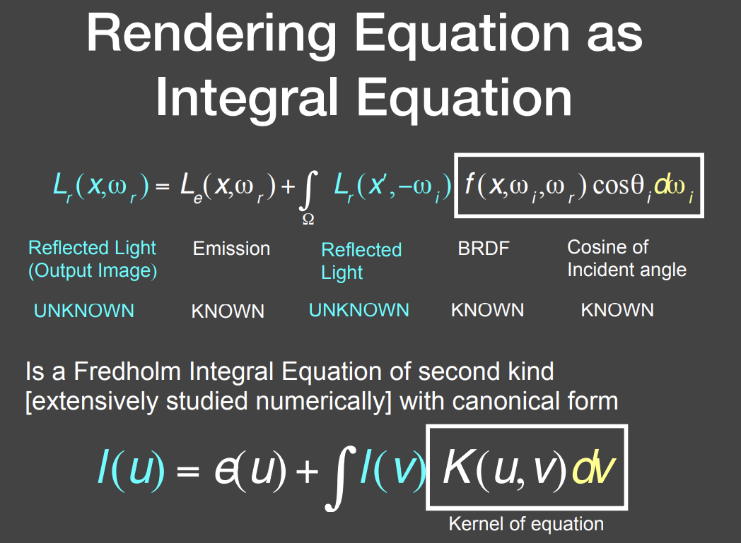
可以把渲染方程进一步简化为一个线性矩阵方程
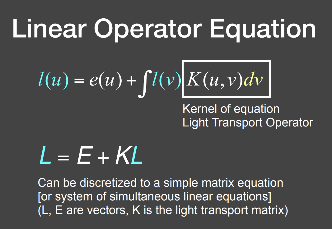
最终就是要把L解出来
写成这么一种算子的形式,因为这个算子同样有类似泰勒展开的性质,虽然是矩阵,但也可以写作这样的形式
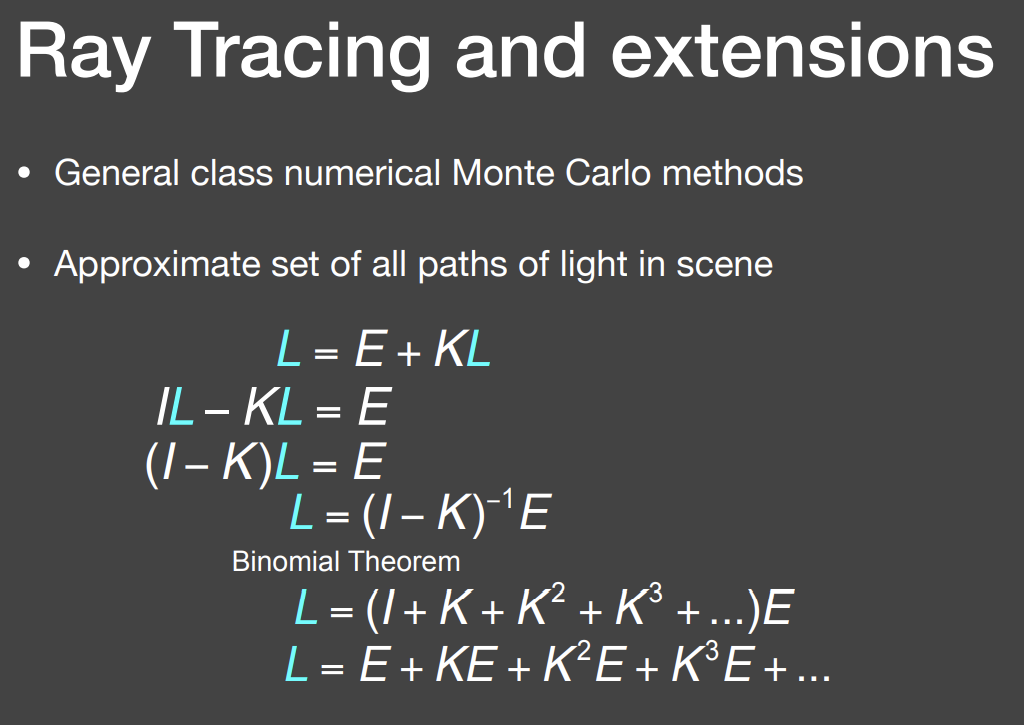
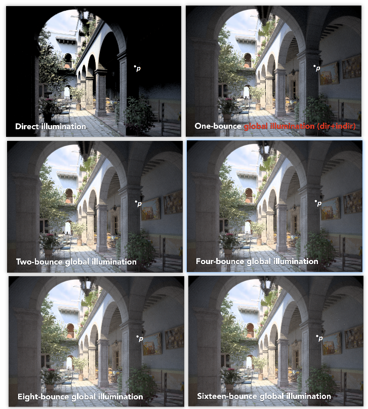
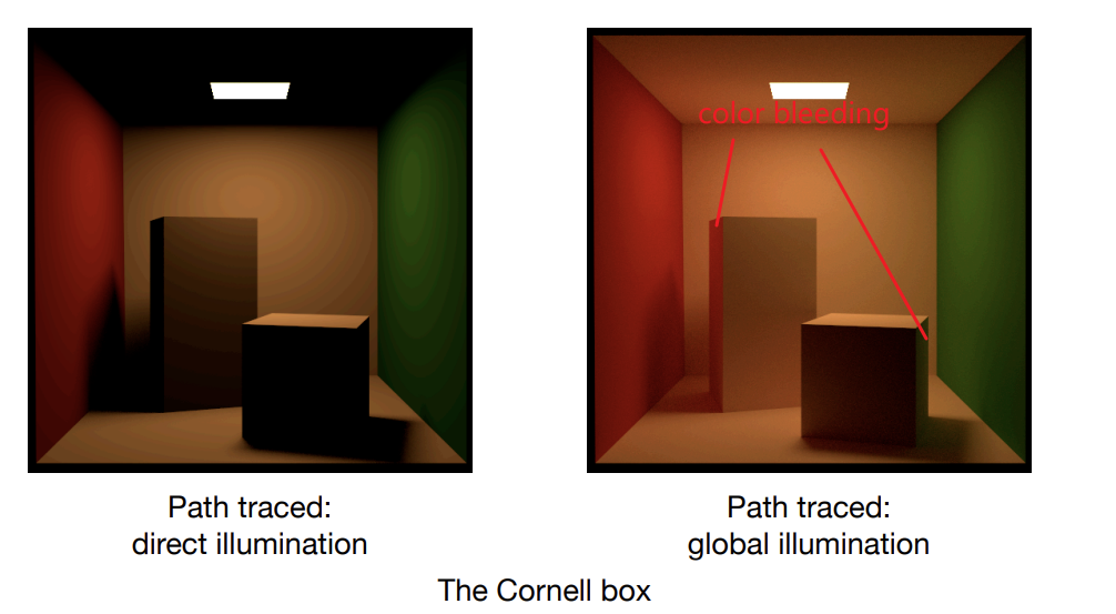
最终看到的能量分解为:直接看到的光源能量(自发光)+光线弹射一次看到的能量(直接光照)+光线弹射两次看到的能量(间接光照)+…(间接光照)…
所有光线弹射的间接光照得到的集合是全局光照
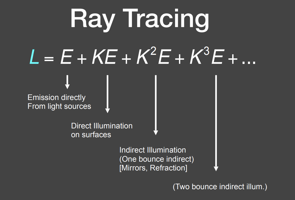
从光栅化的角度来看渲染方程的分解,着色做的就是分解项的前两项,即光栅化能告诉我们的内容就只有自发光和直接光照部分,后面的部分就会比较麻烦
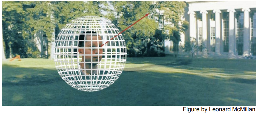
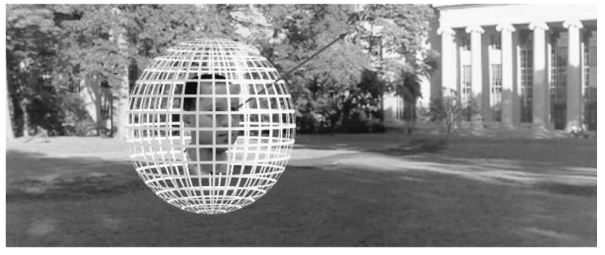
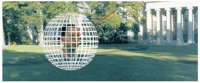
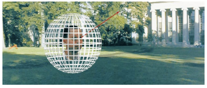
光照弹射次数的效果对比:
路径追踪 Path Tracing
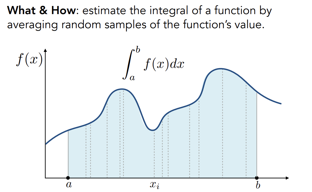
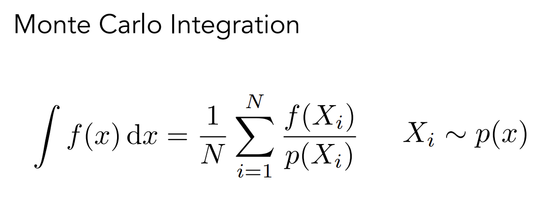
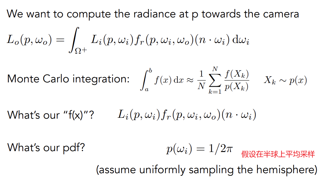
Monte Carlo Integration
What&How
What:解一个定积分:不写出不定积分积分后的解析式,而是直接获得定积分
How:在积分域内不断去采样,把整个积分区域的函数当作是一个矩形(y相等),采样采到的x对应的y就作为整个函数的y,这样多次采样后再求平均
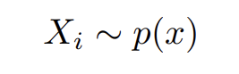
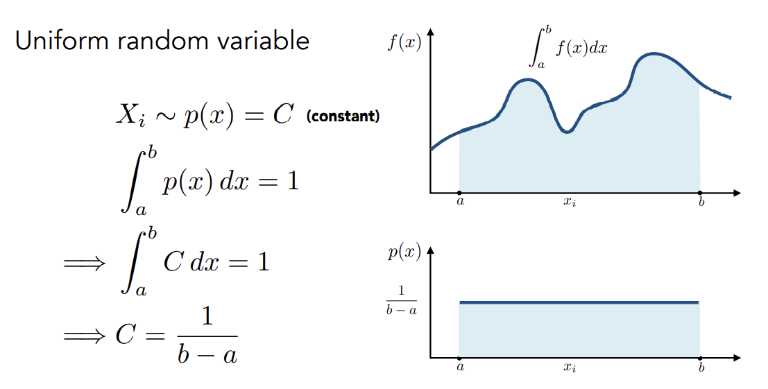
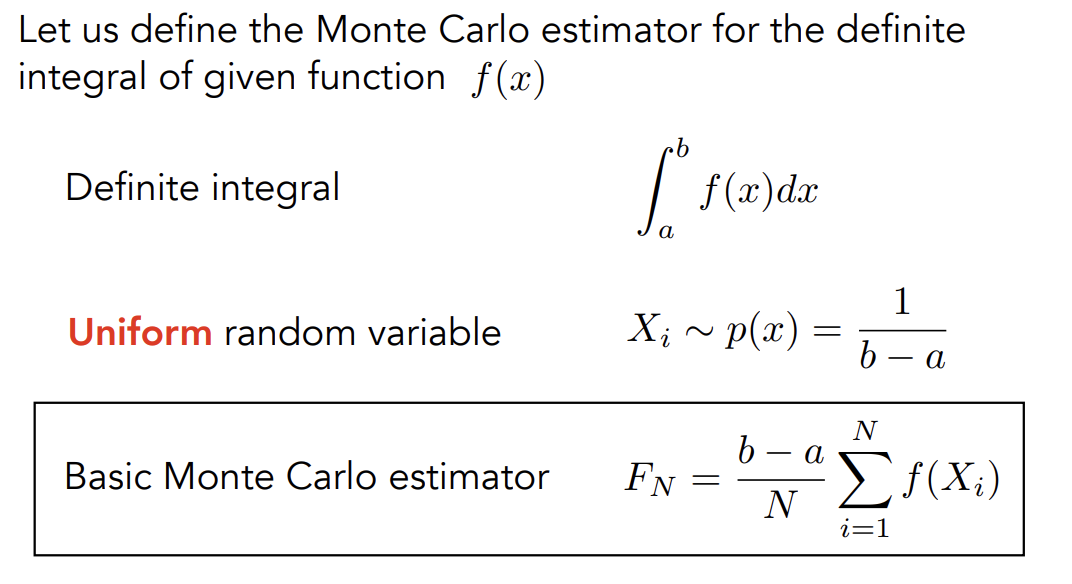
Definition
通过给定的函数定义Monte Carlo Integration
-
Definite integral
-
Random variable
-
Monte Carlo estimator
是采样点在积分域上的概率,即为,所以相当于矩形的宽
如果在[a,b]上平均采样的特殊情况:
note:
- 采样点越多,误差就越小
- 不用关心积分域,在考虑积分时不用考虑积分域是多少,积分域已经在PDF(Probility Distribute Function)中体现出来了
- Monte Carlo积分要求:在x方向上采样,就在x方向上积分
Path Tracing
Problems of Witted-Style Ray Tracing
Problem 1
光线应该被glossy材质(并非完全光滑的材质)反射到哪里
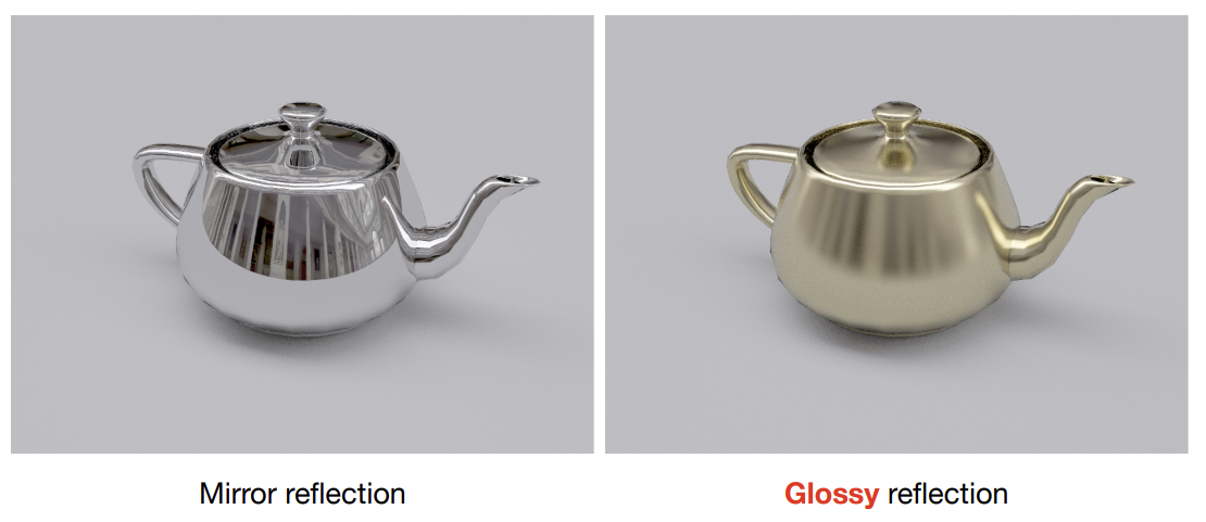
Problem 2
漫反射材质之间的相互反射
Whitted-Style Ray Tracing is Wrong
But Rendering equation is correct
但是这个方程包括:
- 计算在半球上的积分
- 递归计算
A Simple Monte Carlo Solution
假定渲染一个像素在所受直接光照的结果
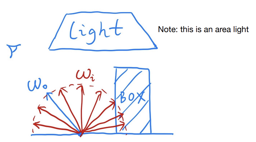
通过反射方程来做解释(因为渲染方程也只是多了一个自发光),那么实际上就只是一个在不同方向上的积分。通过Monte Carlo积分计算就是随机取一个方向作为随机变量,找到他对应的和PDF即可
反射点为p
将积分变为一个简单的求平均值
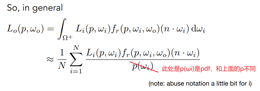
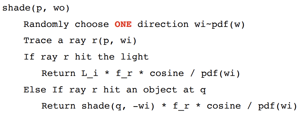
算法:
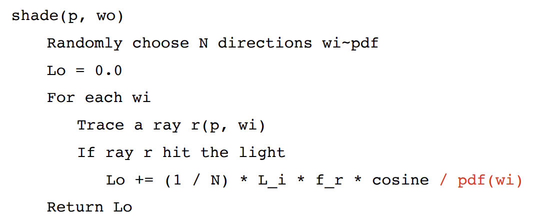
Introducing Global Illumination
加入间接光照就相当于:眼睛在P点看Q点,获得P点的吸收能量
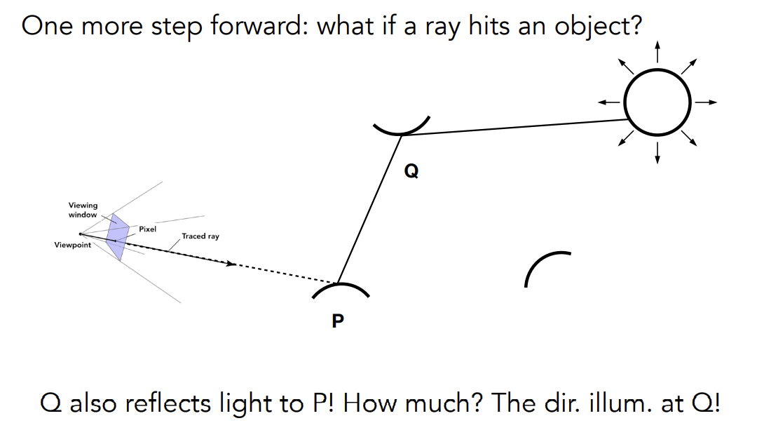
递归算法:
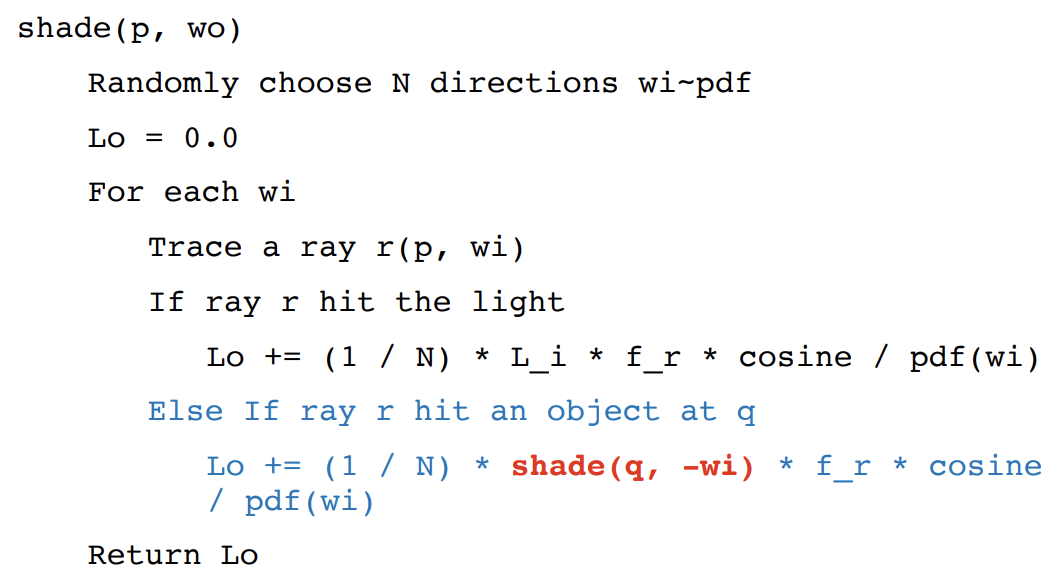
但是存在问题
-
Problem 1:如此计算,光线的数量会“爆炸”
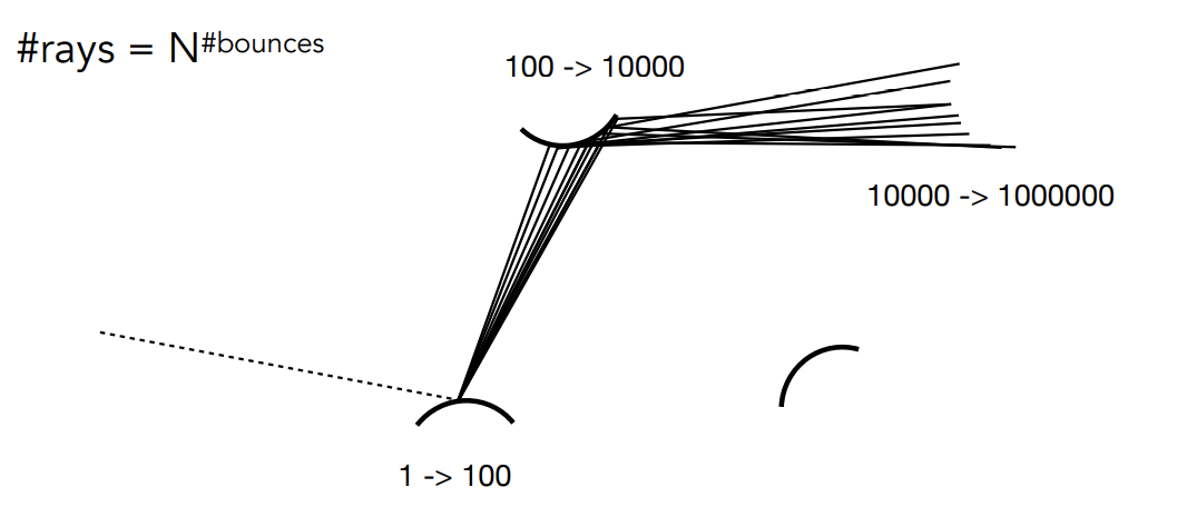
N = 1 唯一能防止指数爆炸
所以进一步改进算法:目前,我们假设在每个着色点上只有一根光线被追踪
用N = 1来做Monte Carlo积分就叫做路径追踪,N != 1叫做分布式光线追踪(光线指数爆炸)
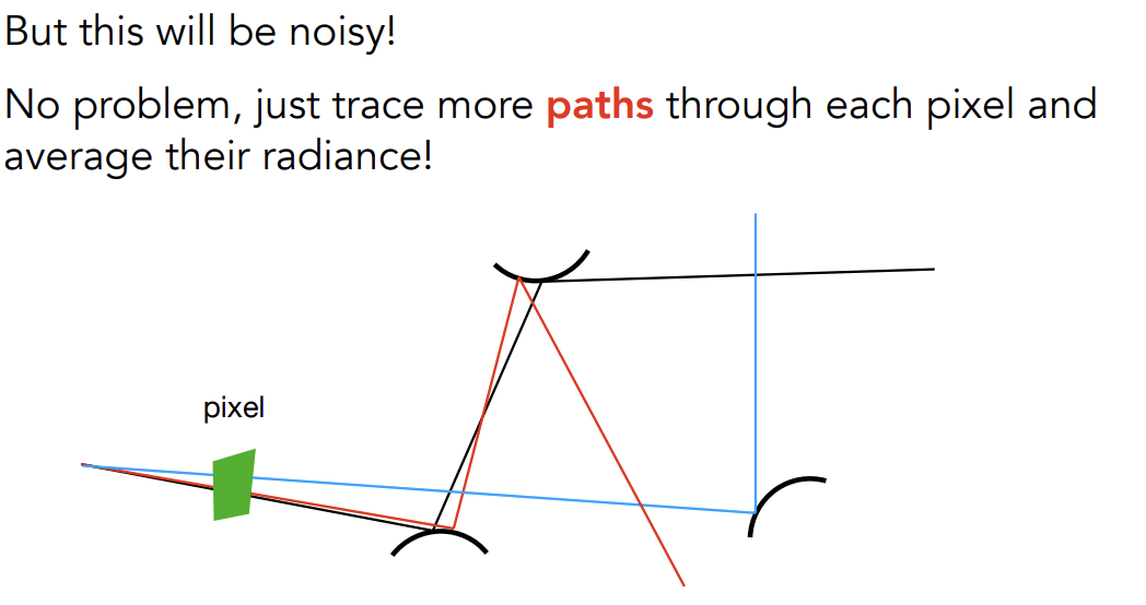
这样获得的结果会变得noisy,不过通过在每个pixel上追踪更多的path(注意不是增加N)并最后取radiance的平均即可
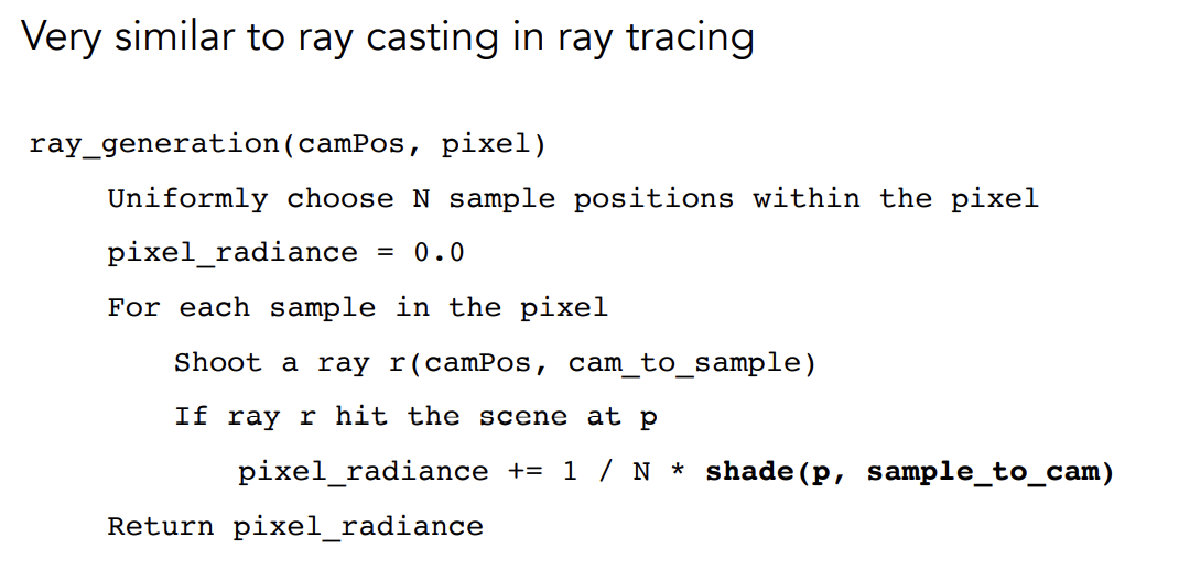
算法:
-
Problem 2:递归算法何时停止?
不能通过限制递归次数的方法来解决,这样做会损失能量,cutting ##bounces == cutting energy,多次弹射的能量就损失了
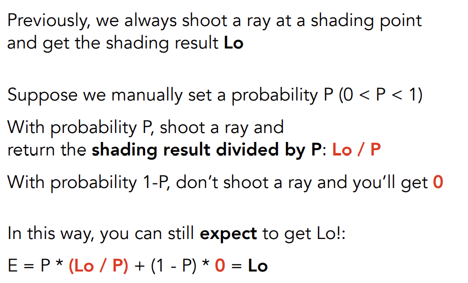
Solution:Russian Roulette(RR)
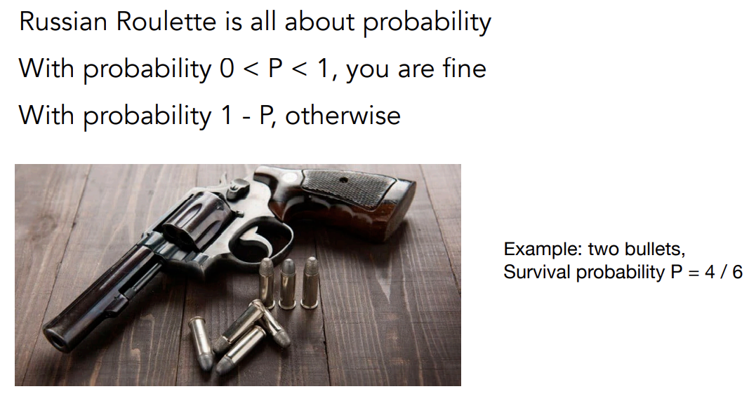
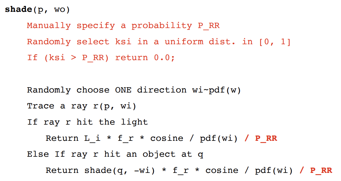
用俄罗斯轮盘赌的方式来决定一定的概率停止向下追踪,即不会一直向下追踪,在一定的条件下会停下来
首先,某一个着色点它的出射的radiance是,给一个概率p,,以一定的概率p向某个方向打一条光线,返回值为得到的一定的结果再除以p,即/P;在1-p的概率内不打出光线,返回0。最终,得到的结果的期望仍然为
代码:
Sampling the Light
以上已经是正确的Path Tracing了
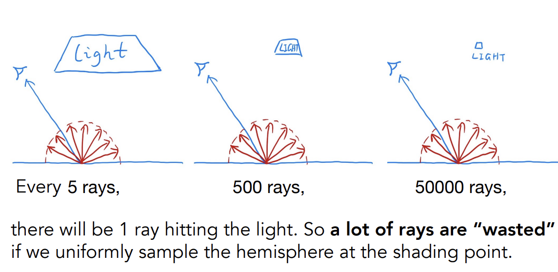
但是这样的Path Tracing并不高效,SPP不足就会出现很多噪点
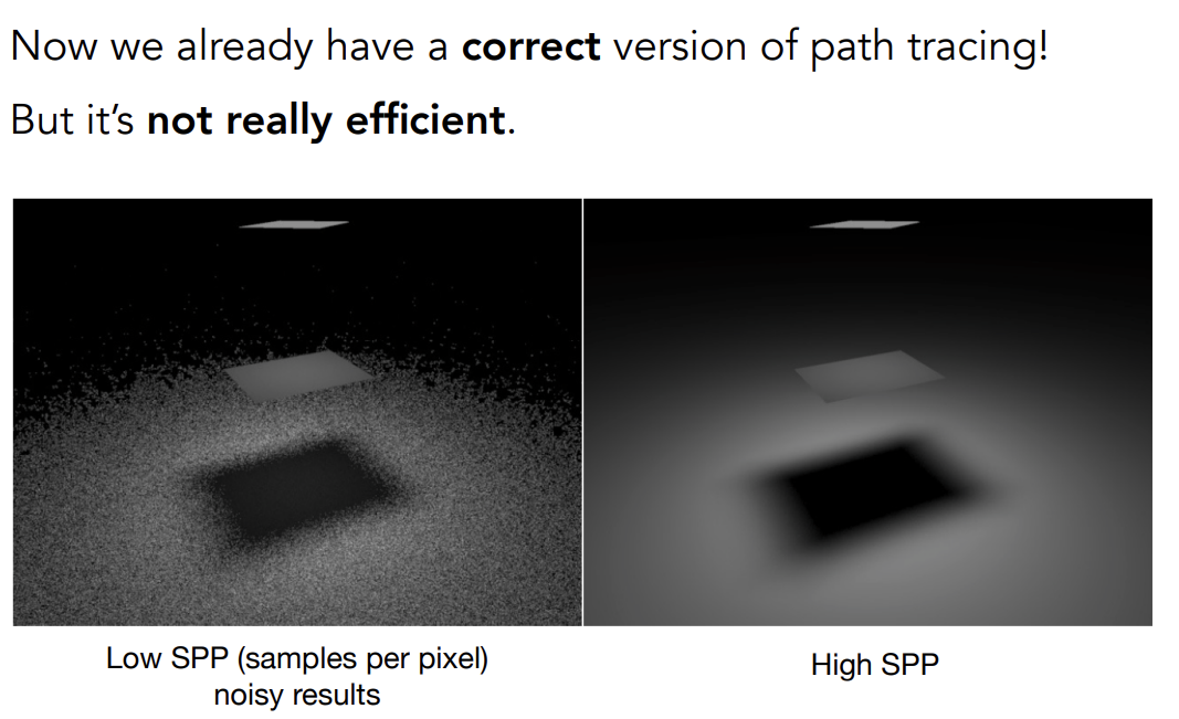
低效的原因:
在着色点上向半球四面八方均匀采样时,从一个点打出去的很多线中只会有1根打到光源,有很多的光线被浪费
Solution:
直接在光源上进行采样要对光源上的微表面面积进行积分把BRDF方程改写成对的积分
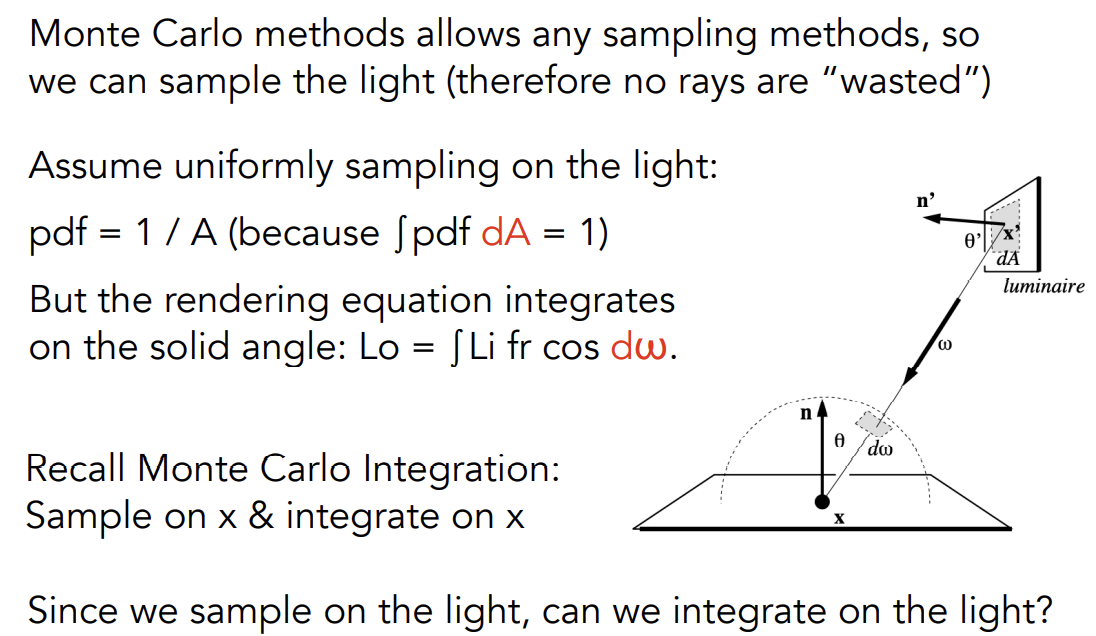
知到和的关系即可——投影的面积
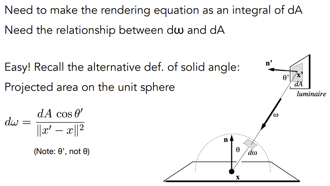
变量替换后:
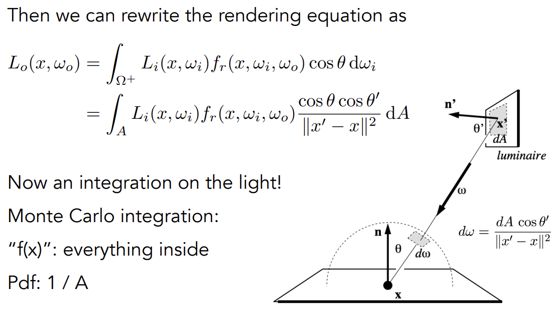
所以可以把着色点接收到的radiance分为两部分:
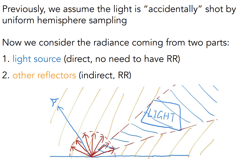
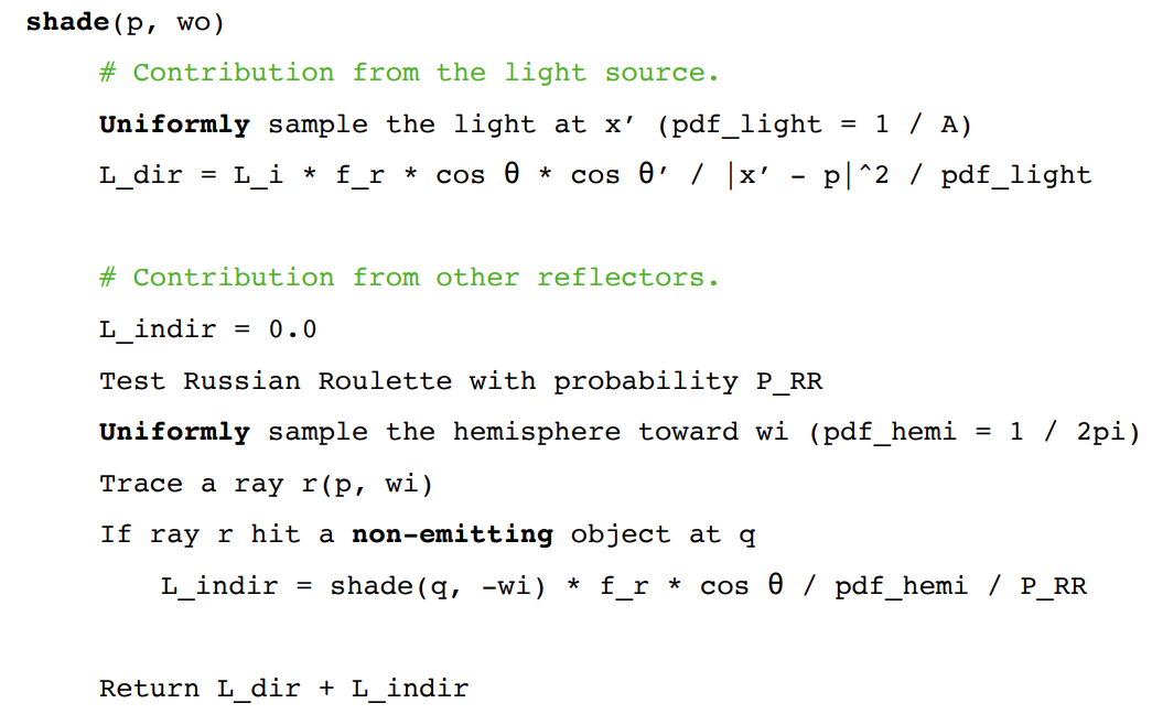
多一步判断光源和接收点p之间有物体阻挡
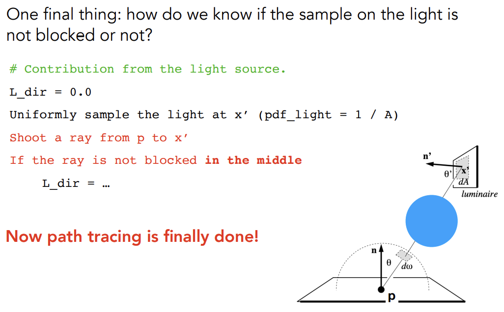
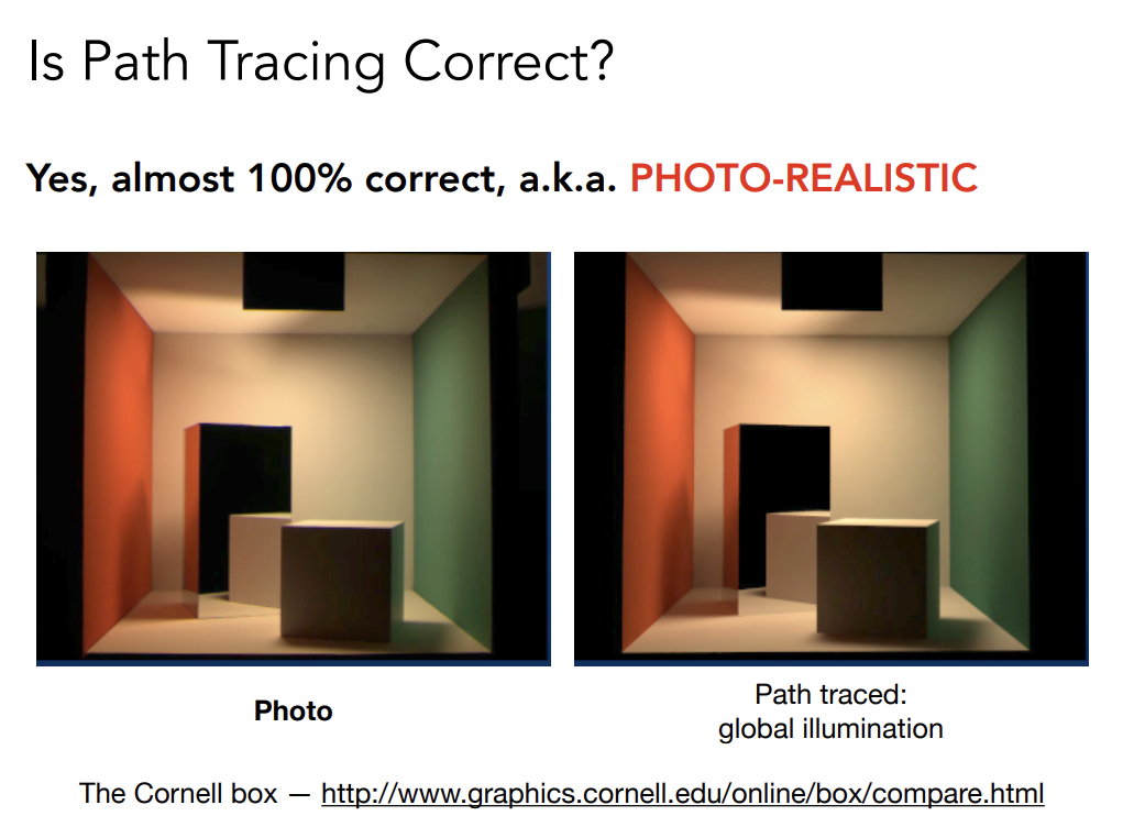
Path Tracing will Generate Photo-Realistic
Some Side Notes
Modern Concepts of Ray tracing
-
Previous
Ray Tracing == Whitted-style ray tracing
-
Modern
The general solution of light transport, include:
- Unidirectional & bidirectional path tracing
- Photon mapping — 光子映射
- Metropolis light transport — 光线传输
- VCM — 结合双向路径追踪和光子映射
- UPBP — 结合所有方法
Haven’t covered
- 怎样对半球进行采样
- Monta Carlo积分能用在任意的pdf上,那么选择什么样的pdf是最好的(importance sampling)
- 随机数的选取(low discrepancy sequences)
- 采样半球和采样光源结合(multiple imp. sampling)
- 对能量的平均是否加权(pixel reconstruction filter)
- 一个像素里面的radiance怎么混合颜色(gamma correction,curves,color space)
材质和外观 Materials and Appearances
Material == BRDF
Diffuse/Lambertian Material(BRDF)
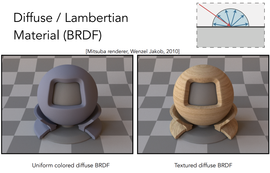
漫反射系数的正确定义:
假设空间中各个方向进来的irradiance都相同(uniform),反射向各个方向的irradiance也都是uniform,且物体表面不吸收光,由能量守恒得到入射光的radiance和出射光的radiance相同,即,所以
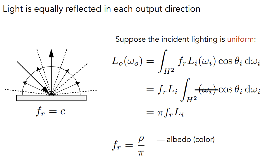
即为albedo:反射率,在0-1之间
Glossy Material
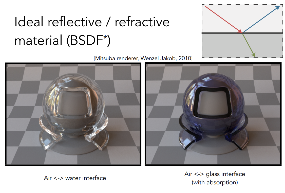
Ideal Reflective/Refractive Material(BSDF)
BSDF = BRDF + BTDF
Perfect Specular Reflection
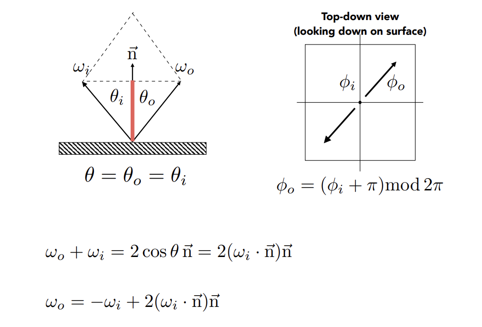
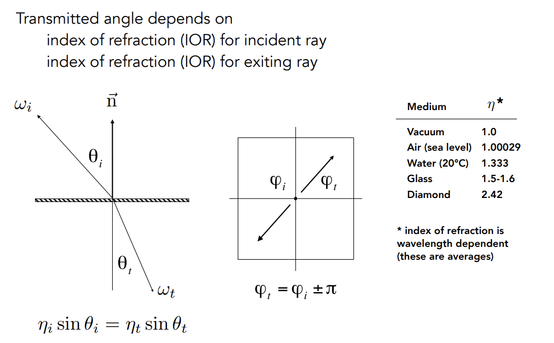
Specular Refraction
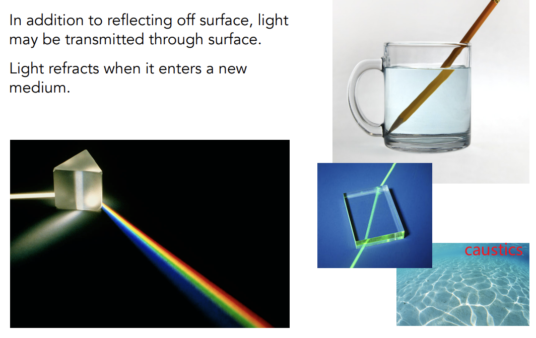
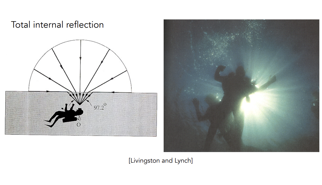
Snell’s Law
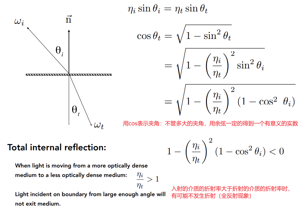
Snell’s Window/Circle
水底只有一个锥形区域会有光线折射进入(只能看到一个锥形区域)
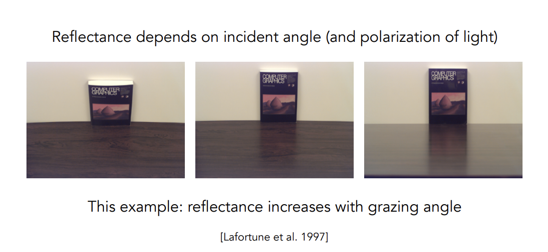
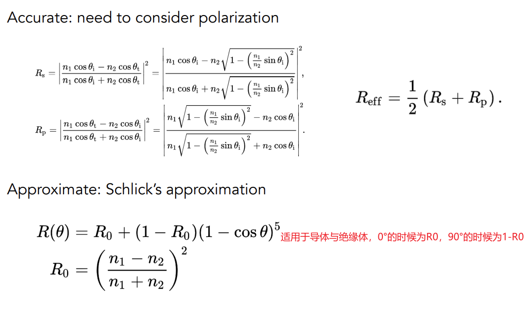
Fresnel Reflection/Term
现象:不同角度看桌面,反射内容是不一样的
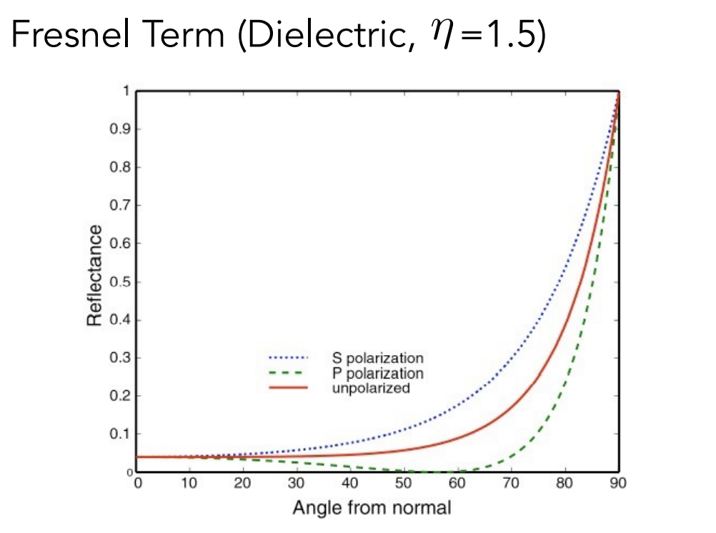
菲涅尔项:
-
绝缘体反射率随入射光角度变化
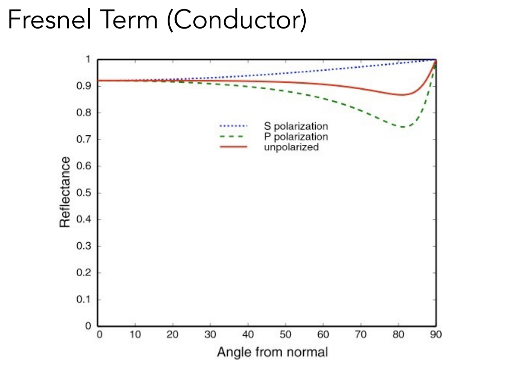
-
导体反射率随入射光角度变化
-
计算公式
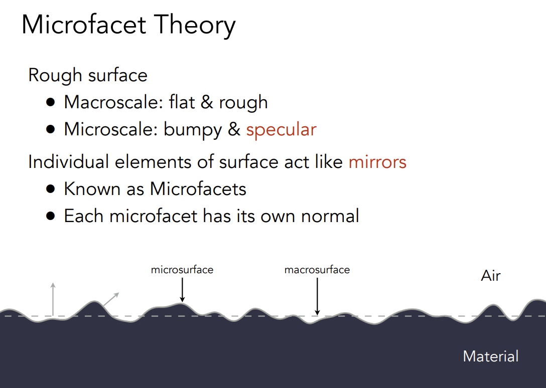
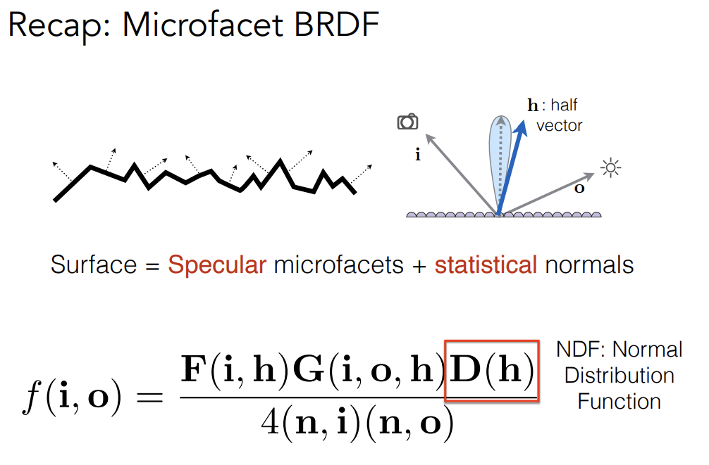
Microfacet Material
Microfacet Theory
粗糙表面:
- Macroscale:flat&rough(从近处看的是几何)
- Microscale:bumpy&specular(从远处看的是材质)
单个微表面都想一面镜子一样
- 每个微表面都有自己的法线(朝向)
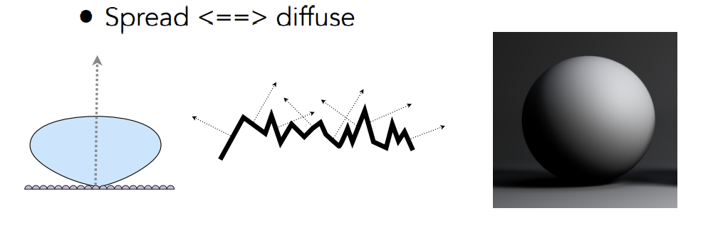
Microfacet BRDF
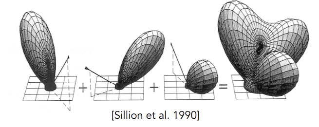
-
key:研究微表面发现的分布
-
微表面分布集中glossy

-
微表面分布分散diffuse
-
-
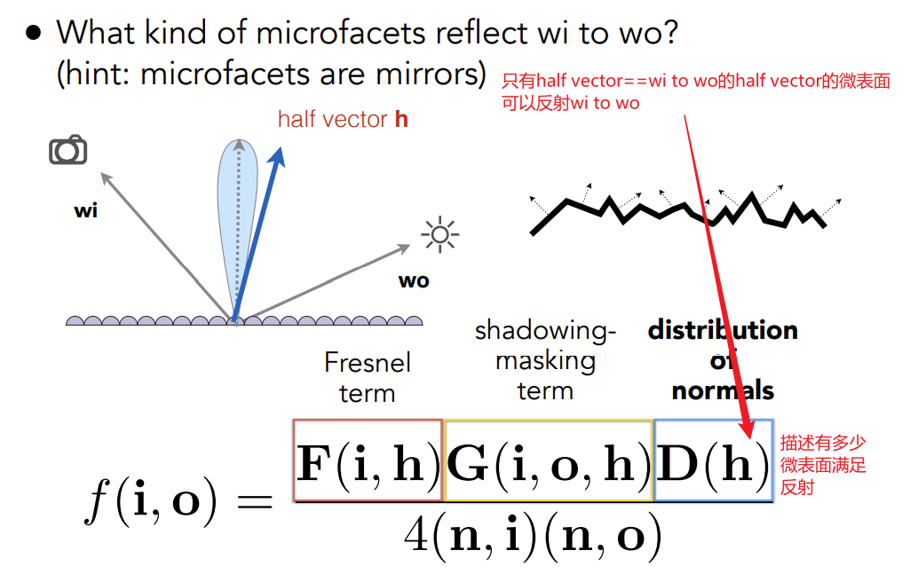
Microfacet BRDF
-
—— shadowing-masking term
微表面之间可能发生相互遮挡,所以有些微表面满足反射但是会被遮挡,失去了他们的作用,即实际计算得到的反射能量可能偏大。Shadowing-masking考虑的就是这个现象。定义一个Grazing Angle,十分接近与法线垂直的角度,当光线接近Grazing Angle时,shadowing-masking就用于修正这个现象。
-
—— distribution of normals
描述有多少微表面实现从入射到出射方向的反射
-
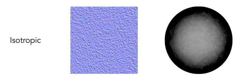
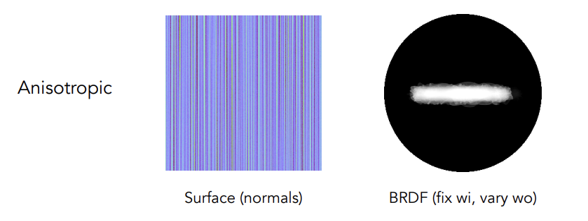
Isotropic/Anisotropic Materials
-
Key:directionality of underlying surface
-
各向同性:认为微表面并不存在一定的方向性或方向性很弱,微表面的发现分布均匀
-
各向同性:微表面有一定的方向性
-
-
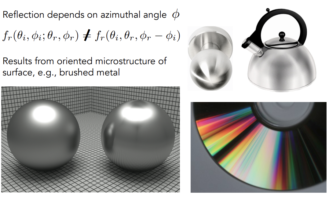
Anisotropic BRDF
旋转反射的方位角(azimuthal angle),如果观测到的BRDF不变,那么说明是各向同性;如果观察到的BRDF发生变化,那么说明是各向异性(BRDF与绝对方位角有关)
Properties of BRDFs
-
Non-negativit
-
Linearity
-
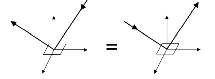
Reciprocity principle
-
Energy conservation
-
Isotropic vs. anisotropic
-
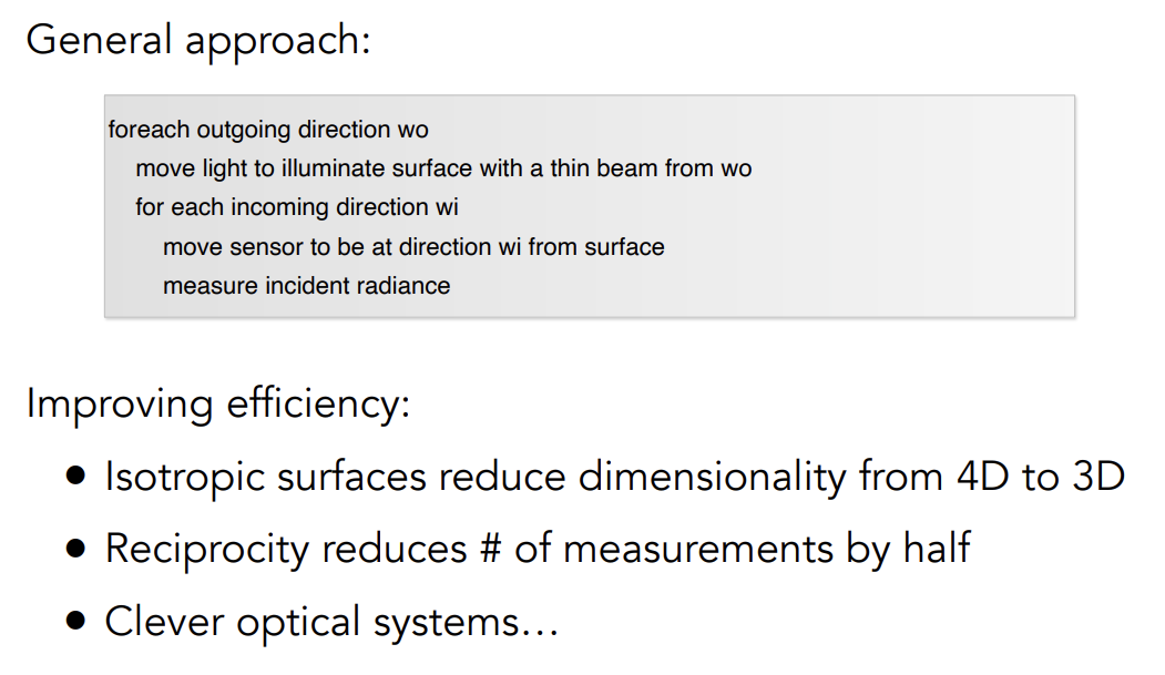
If isotropic,,四维降三维
-
Then, from reciprocity,
由可逆性得,相对方位角不需要考虑正负,方便BRDF的测量和储存
-
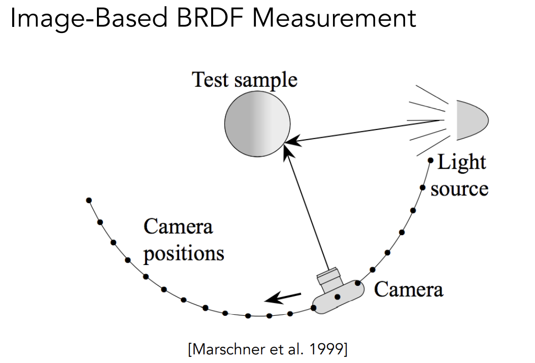
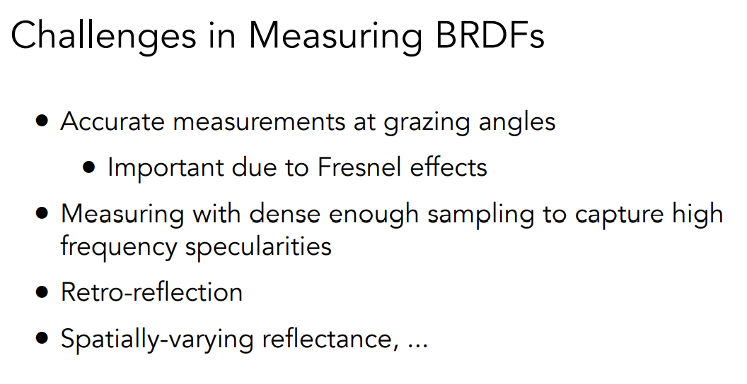
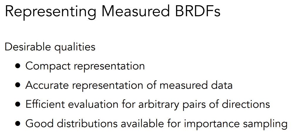
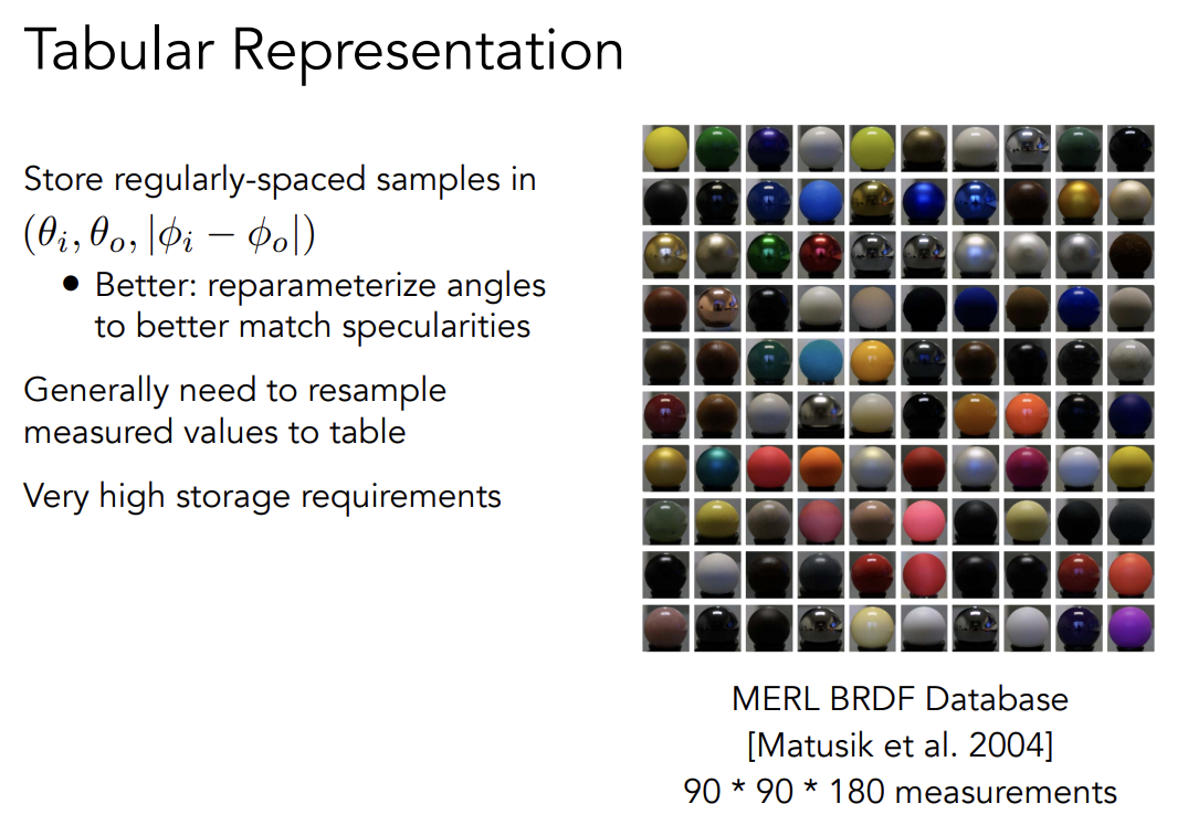
Measuring BRDF
Advanced Light Transport
Unbiased light transport methods
Biased vs. Unbiased Monte Carlo Estimators
-
无偏蒙特卡罗积分不会产生任何逻辑错误
不管用多少采样点,无偏估计的期望值往往是真实值,这样的方法叫做无偏方法
-
有偏:其他情况
特例:期望值在无限多的采样点的情况下收敛于某个值,这样的情况叫做consistent
-
渲染中的biased和consistent的理解
- Biased == blurry
- Consistent == not blurry with infinite samples
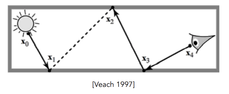
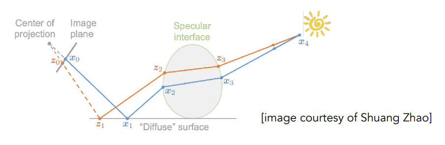
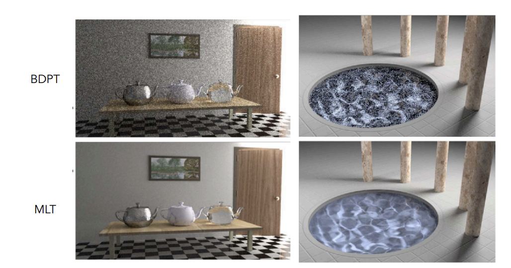
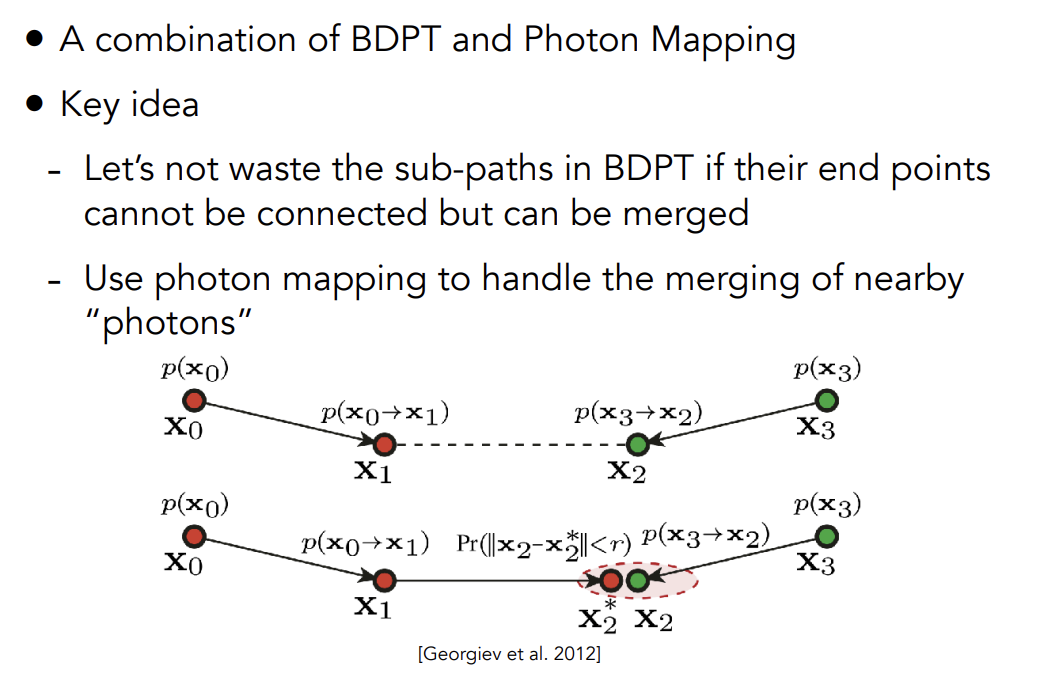
Bidirectional Path Tracing(BDPT)
生成从摄像机和光源出发的子路径,再把两个子路径的端点连接起来的方法
-
适用于光线传播在光源处比较复杂的情况
-
但是实现起来会很难,并且很慢
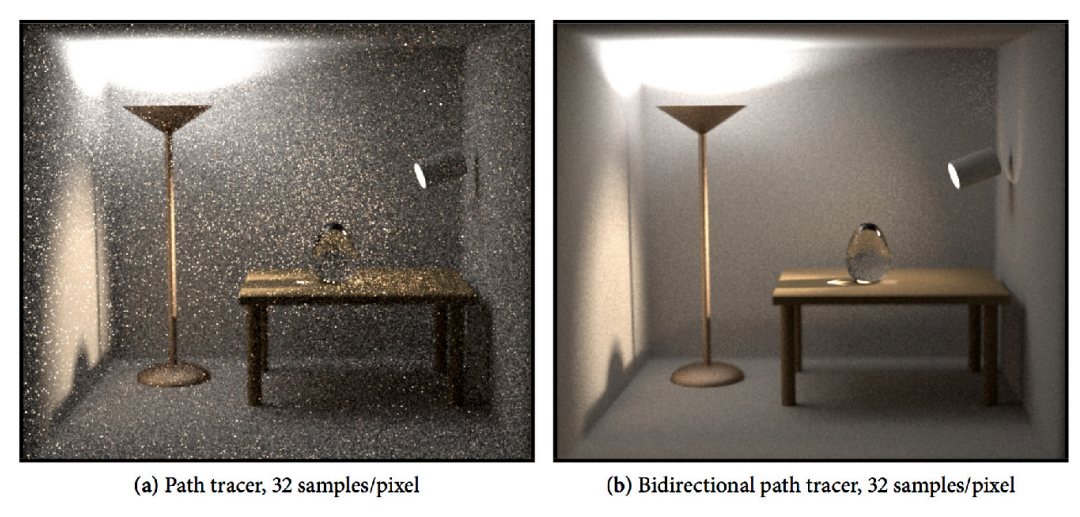
如图,因为Path Tracing从摄像机出发时的第一次bounce是diffuse,导致不好控制它能够打到之后能量集中的地方去,所以效果不好。而Bidirectional Path Tracing可以直接连接光源出发的和摄像机出发的第一次bounce
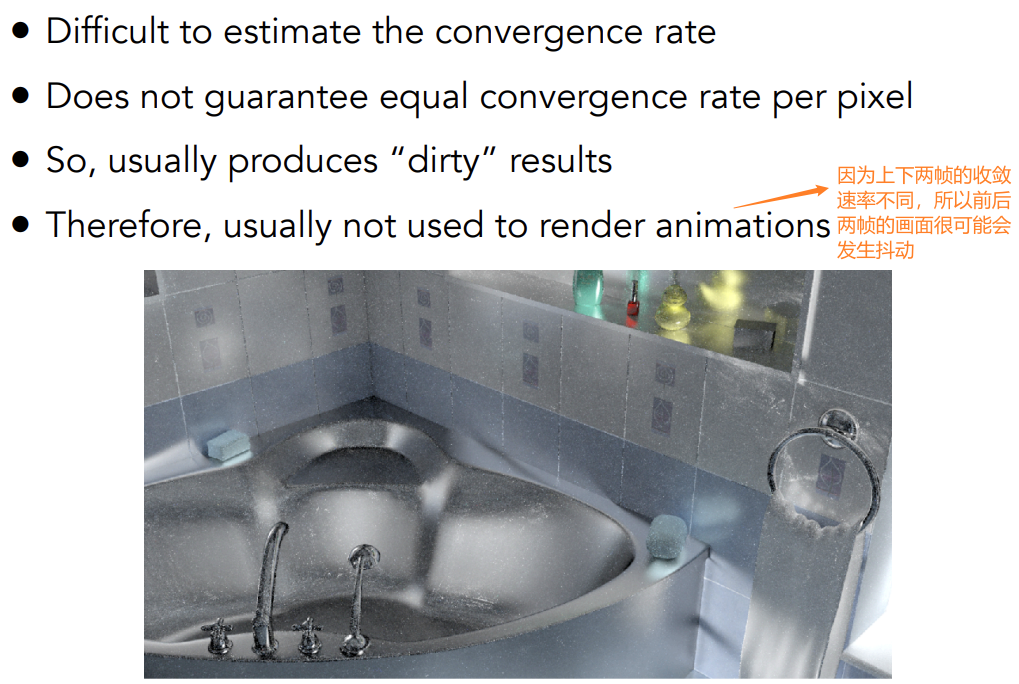
Metropolis Light Transport(MLT)
-
A Markov Chain Carlo (MCMC) application
MCMC可以生成以任意函数的形状为PDF的样本,Monte Carlo Estimator中当你采样的PDF和被积函数形状一致时(和),得到的variance最小。Markov Chain能够让任何未知的函数生成一系列分布与被积函数形状一致的样本。
-
Very good at locally exploring difficult light paths
-
Key idea :
-
Locally pertub an existing path to get a new path
-
-
特别适合做复杂的光线传播
-
只需要找到一条“种子”路径
-
caustics:specular-diffuse-specular
-
-
难以在理论上分析最终的收敛速度(难以估计sample数量和variance的关系)
Biased light transport methods
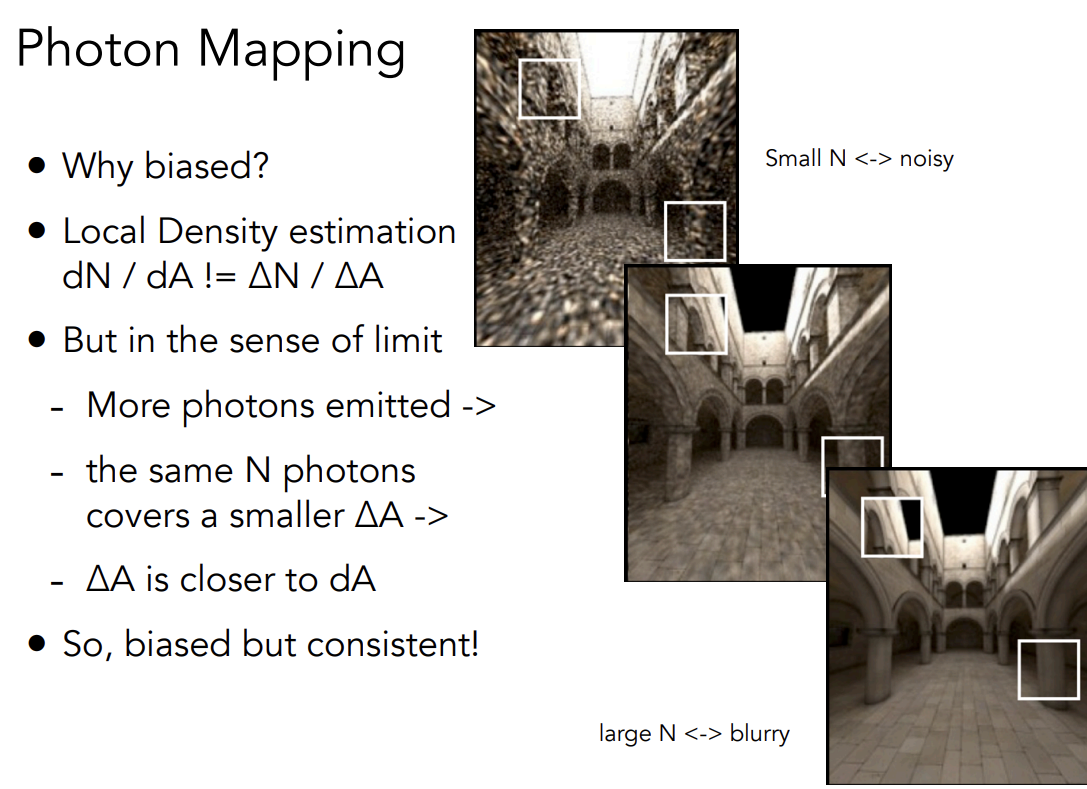
Photon Mapping
-
Very Good at hanging Specular—Diffuse—Specular(SDS) path and generating caustics
-
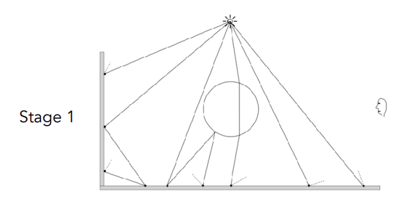
A two-stage method
-
Stage 1 — photon tracing
光子从光源出发,该反射就反射该折射就折射,直到光子遇到一个diffuse材质的物体,光子就停在那里
Stage 2 — photon collection
从视角出发,发射子路径,该反射就反射该折射就折射,直到路径打到diffuse材质的物体上
-
-
Calculation — local density estimation
- areas with more photons should be brighter
- 对于每一个shading point,寻找它周围最近的N的光子,划分这几个光子占据着色点周围的面积,用光子数量除以面积获得光子密度
-
为什么光子映射phonto mapping是有偏的
- Local Density esitimation
- 当有足够多的光子时,
- 所以光子映射biased但是consistent
Vertex Connection and Merging(VCM)
- 结合BDPT和Photon Mapping
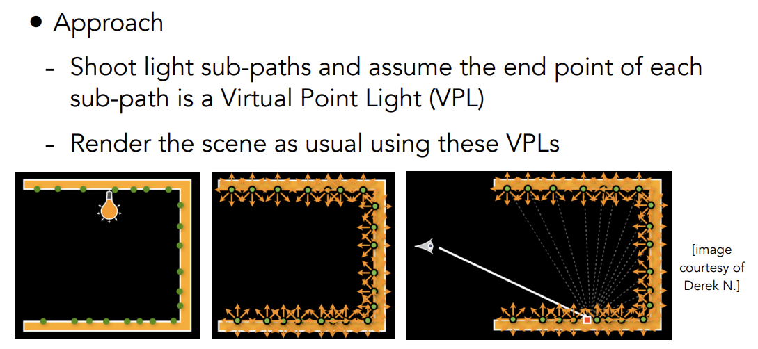
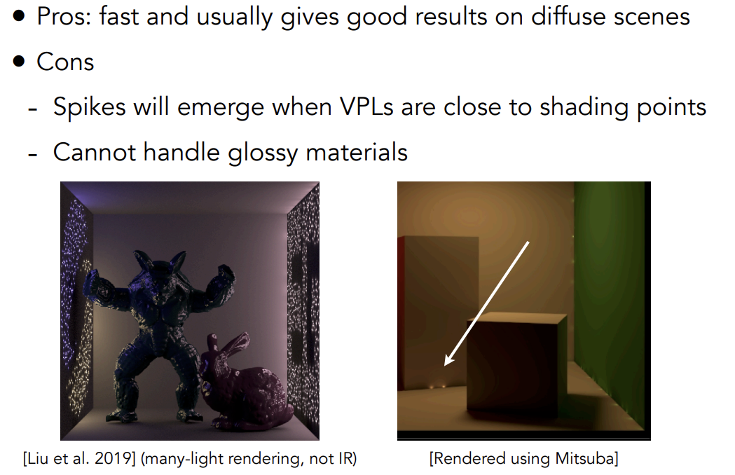
Instant Radiosity(IR)
-
也叫many-light approaches
-
核心思想:把被照亮的表面看作是新的光源
Advanced Appearance Modeling
Non-surface models
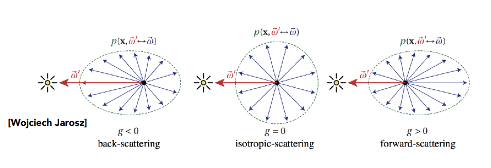
Participating Media
Participating Media: 参与介质
- 光线在参与介质中会发生①被吸收②被散射
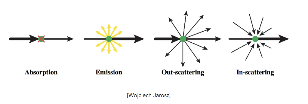
-
使用Phase Function相位函数来描述光在参与介质中任意位置的散射角度的分布情况
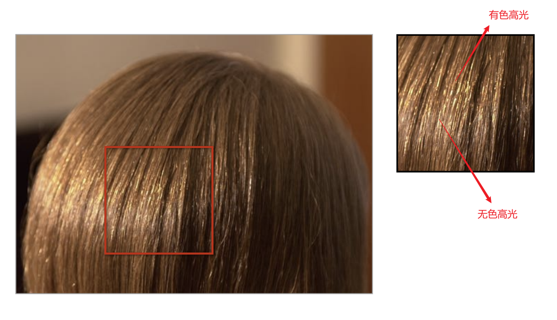
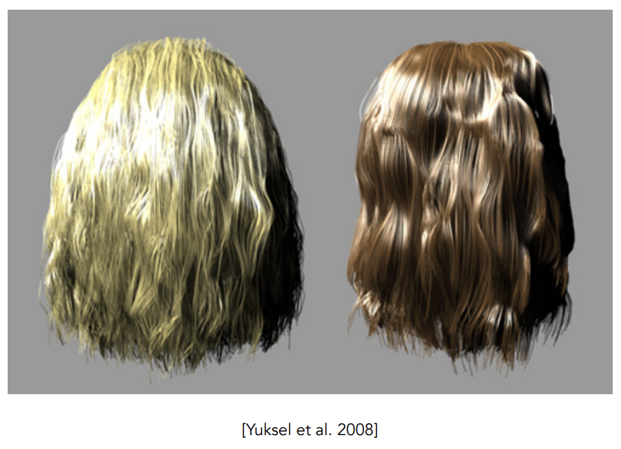
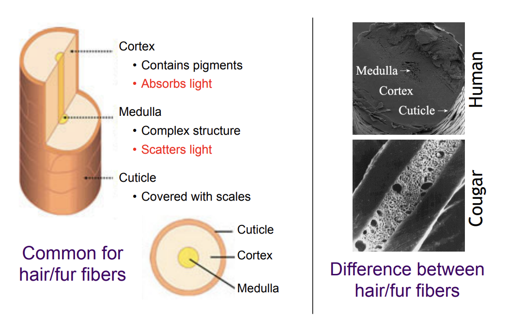
Hair/Fur Fiber (BCSDF)
Human Hair
-
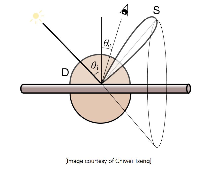
Kajiya–Kay Model
只考虑反射和漫反射
-
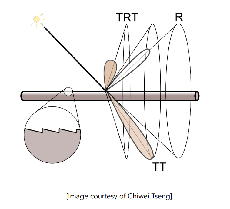
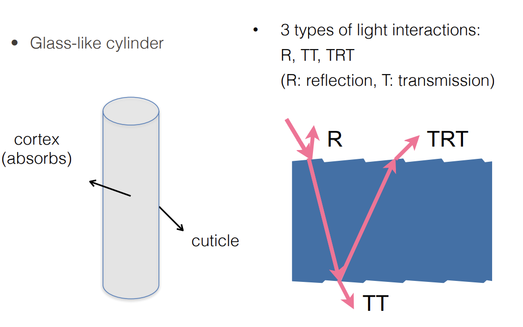
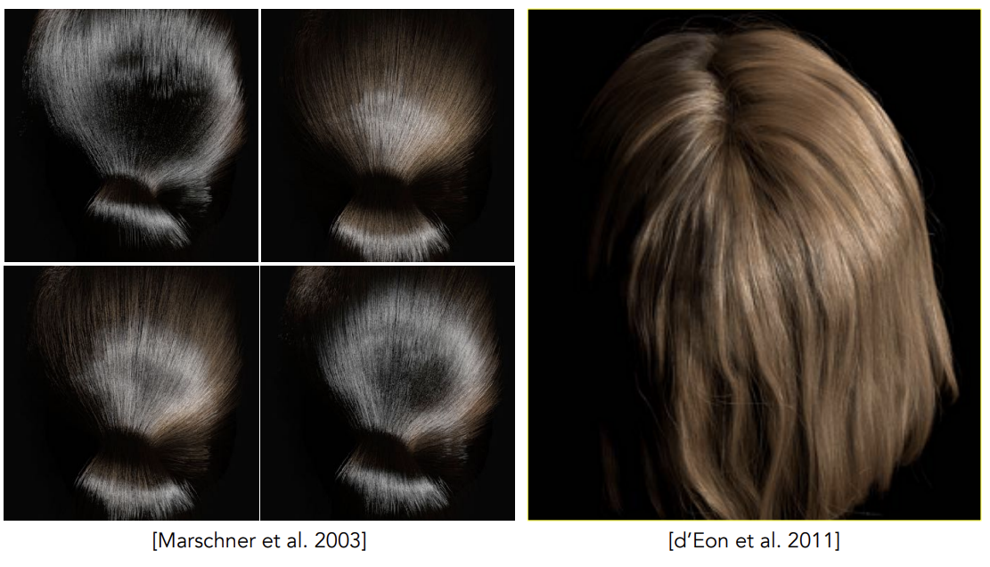
Marschner Model
光线打到圆柱后
有一部分被直接反射——R
有一部分会穿透后再穿透——TT
有一部分进头发里,在内部反射后再发生第二次穿透——TRT
Fur Appearance
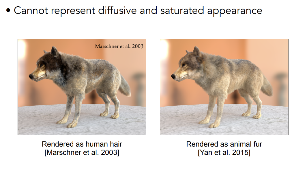
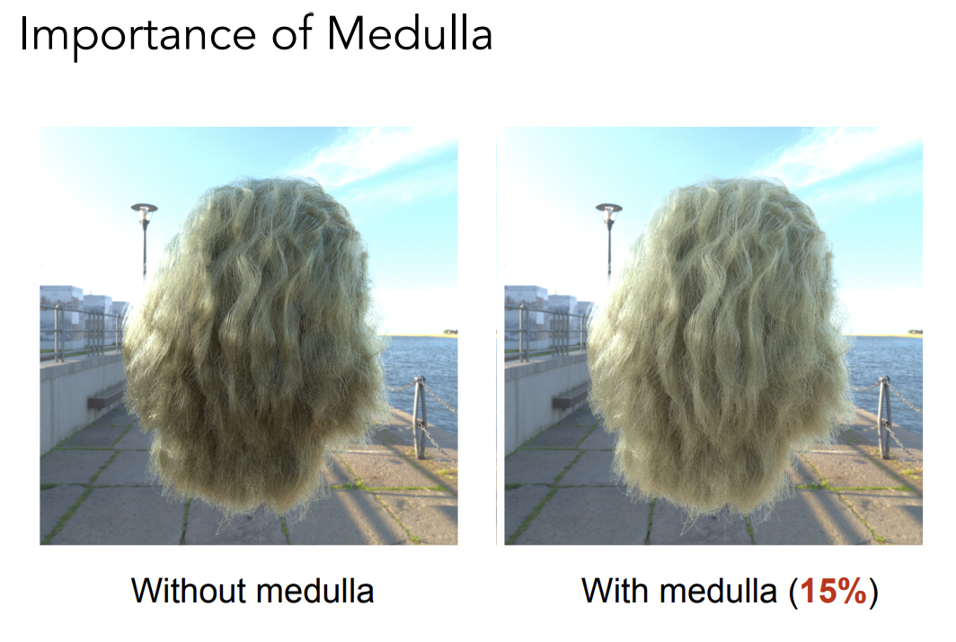
动物毛发不能通过人头发的方式进行计算:动物毛发内的髓质比头发的大得多,之前的玻璃柱的模型没有考虑髓质的存在
-
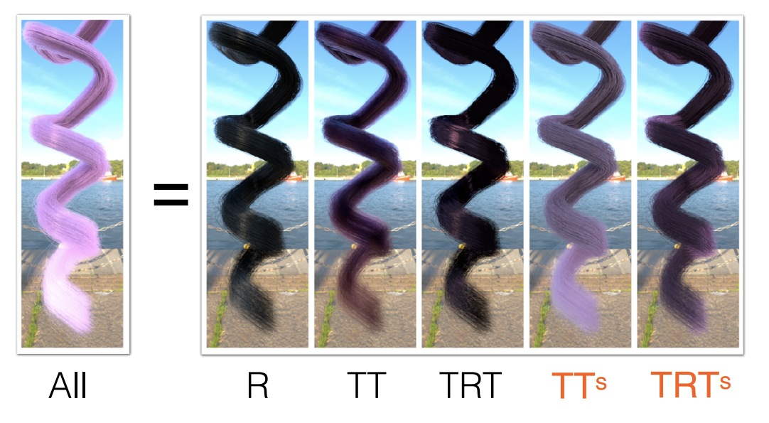
Double Cylinder Model——模拟出髓质
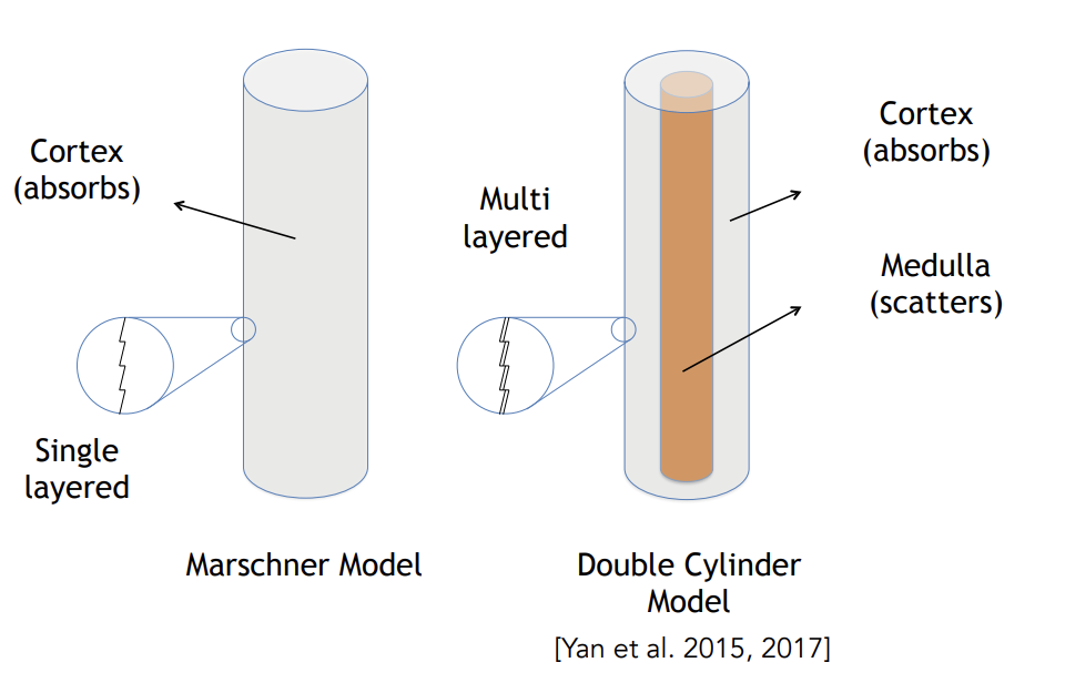
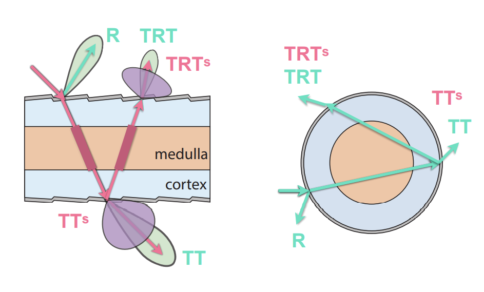
一共五个分量
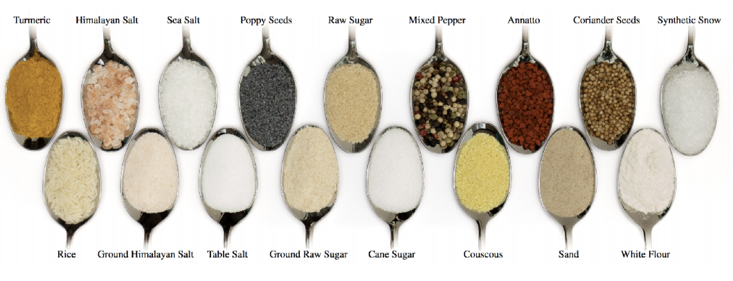
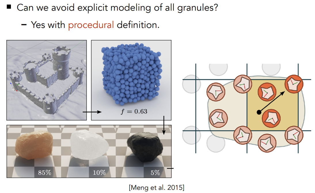
Granular material
颗粒材质
Surface models
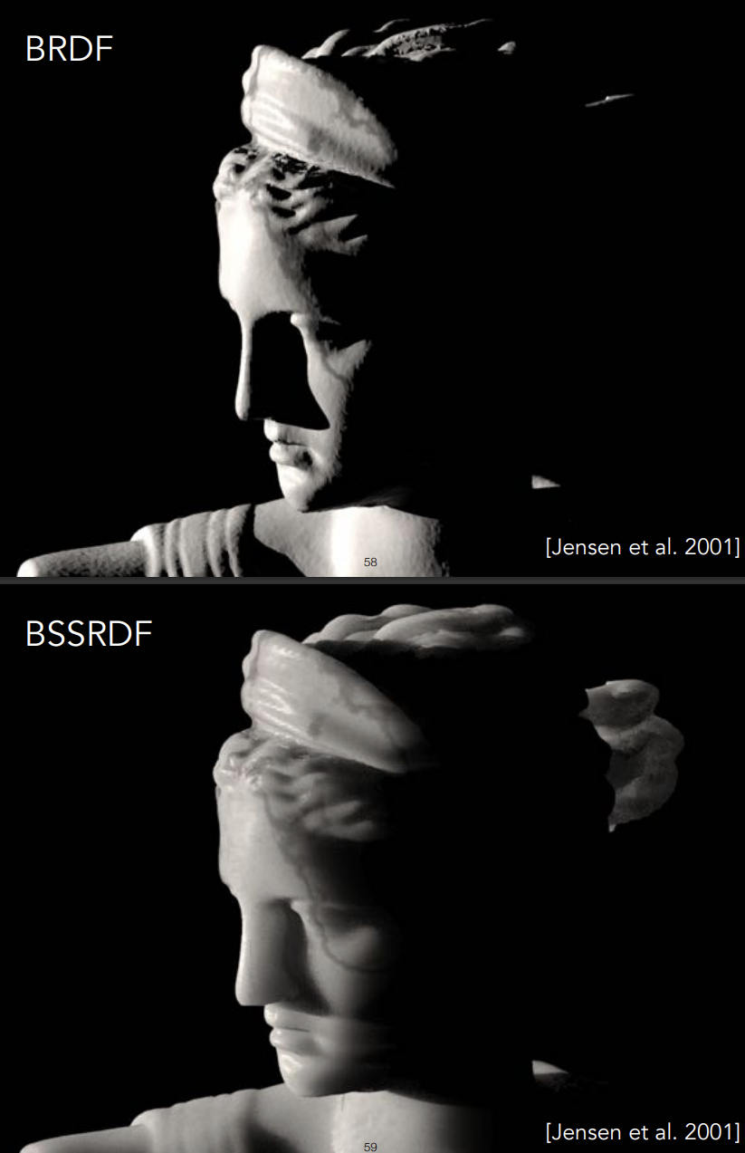
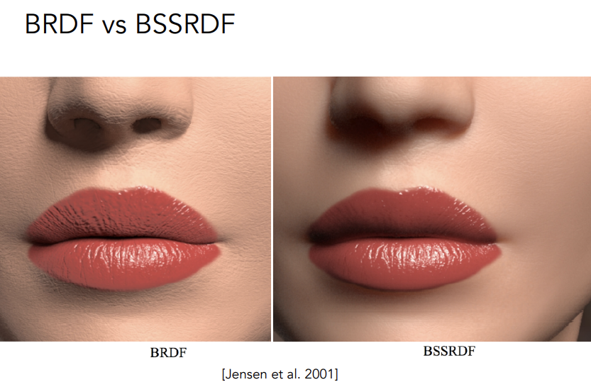
Translucent Materials(BSSRDF)
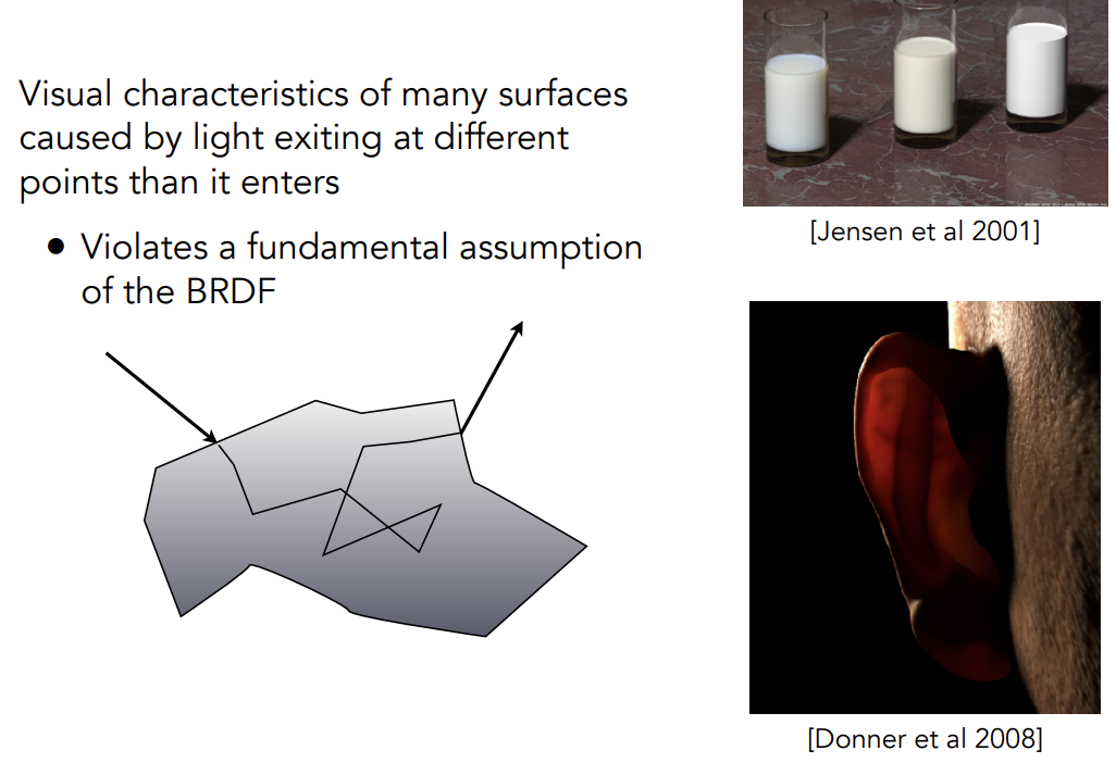
Translucent Materials不是实际的半透明,Semitransparent Materials才是半透明
Translucent Material说明的是光线可以从某一个地方进入物体表面,再从另一个地方出物体表面,并非光线传入一个表面并不被吸收,光线可以被导到其它地方去
-
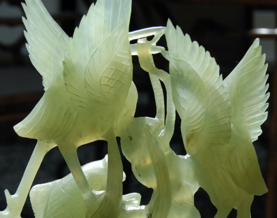
Jade
-
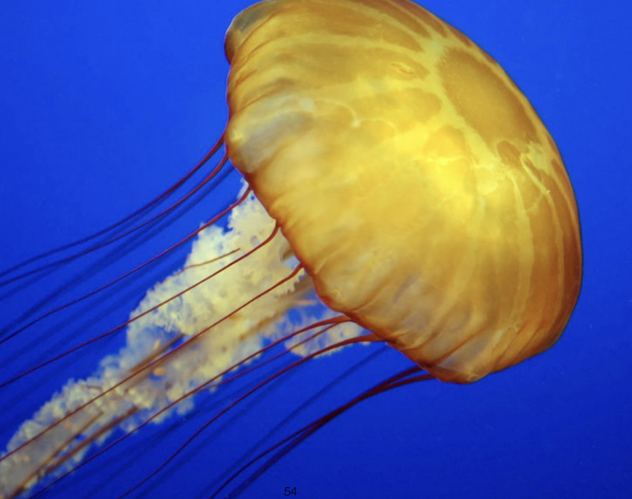
Jellyfish
-
Subsurface Scattering次表面散射
-
Scattering Functions
-
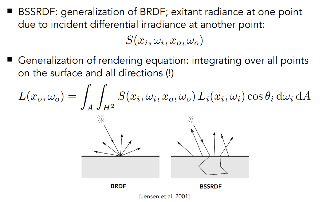
BSSRDF:对BRDF概念的延申
-
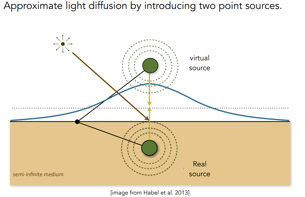
Dipole Approximation
当光源照向一个点后,将BSSRDF近似为物体表面内外两个光源共同照亮这一部分的着色点
-
BSSRDF的效果:
-
Cloth
Rendering as Surface
通过给定的编织模式,计算整体的表现,通过BRDF进行计算
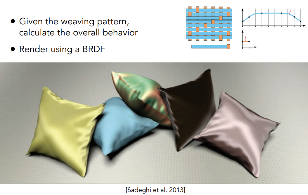
不便于处理anisotropic
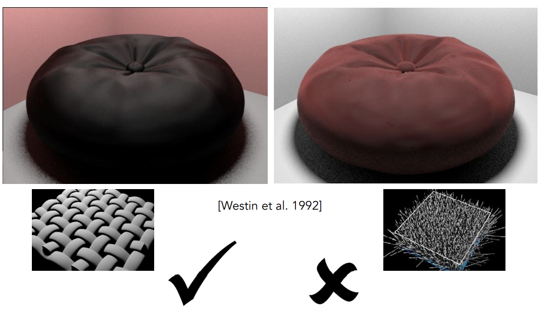
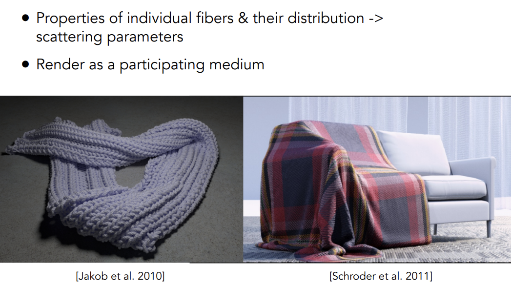
Rendering as Participating Media
不再把布料当作平面渲染,而是当作体积渲染,可以得到更好的效果,但是渲染的计算量就会大得多
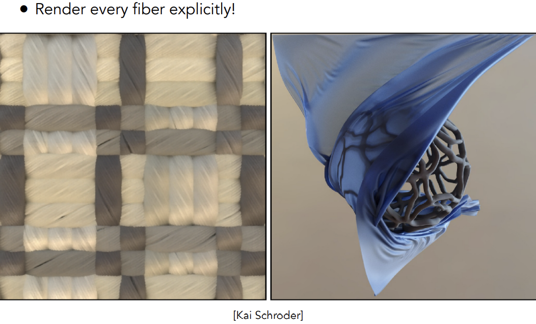
Rendering as Actual Fibers
精确渲染每一根纤维
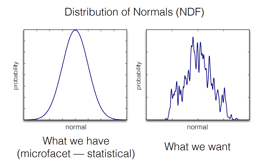
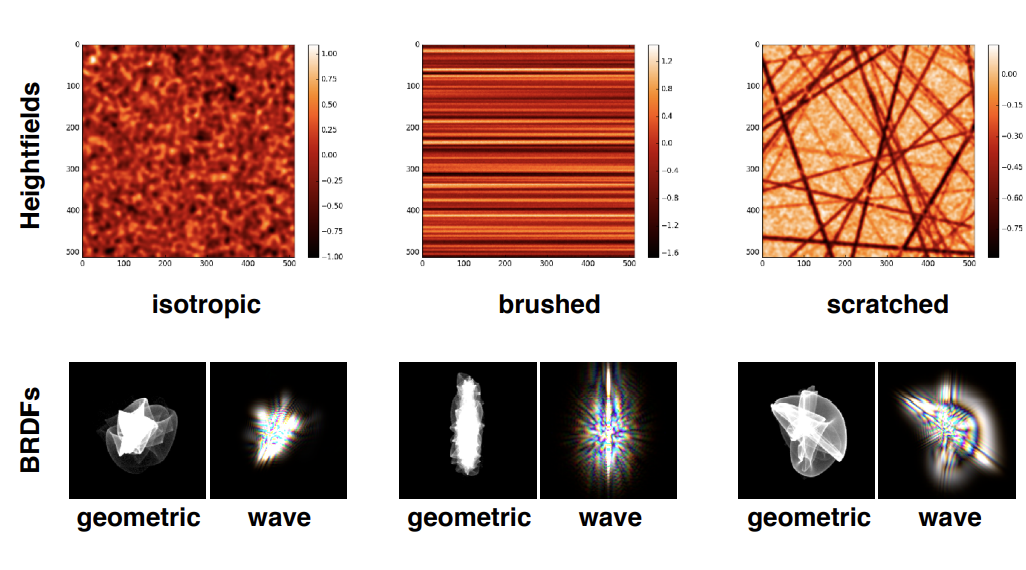
Detailed materials(non-statistical BRDF)
Microfacet BRDF
Normal Distrubution Function(NDF)的不同——实际的NDF存在一些细节,如果能将这些细节考虑进去那么就能得到更好的细节
-
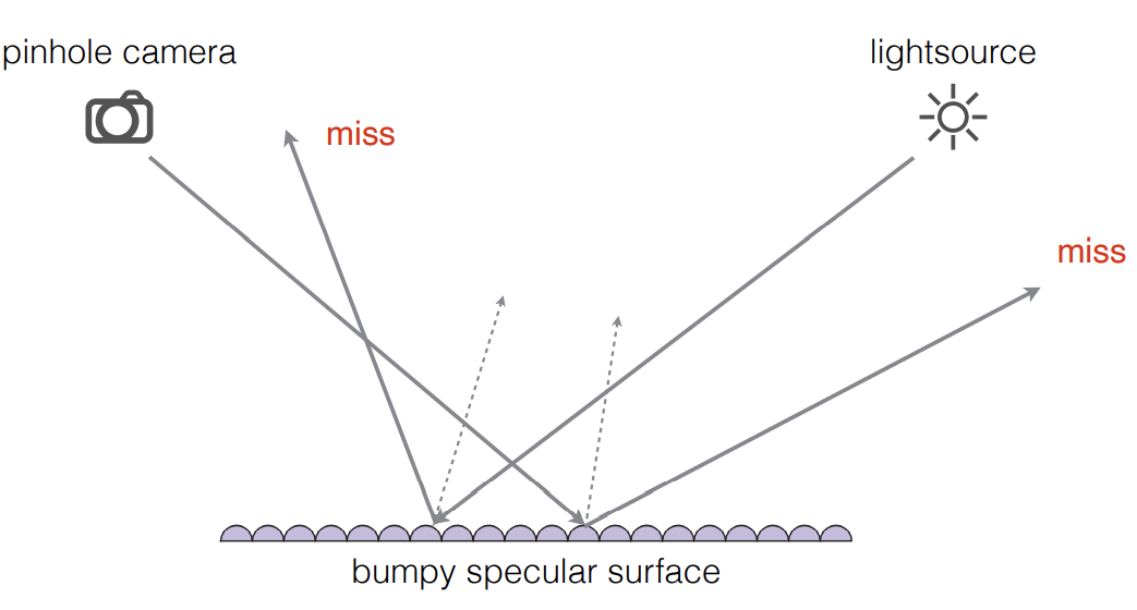
微表面在path tracing上会存在一些问题
- 容易发生path的miss
-
Solution:
考虑一个像素会覆盖很多的微表面,把一个微表面在一个像素对应范围内的法线分布算出来,替代原本光滑的分布并用在微表面模型里
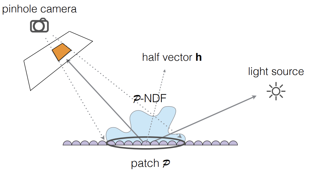
不同大小的patch
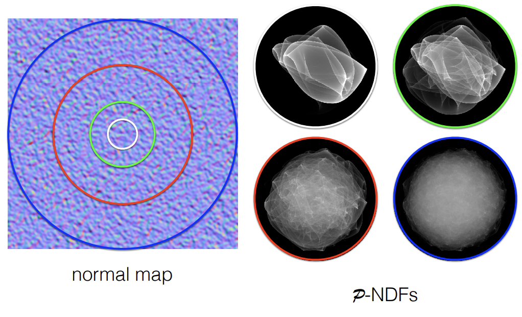
不同的法线贴图
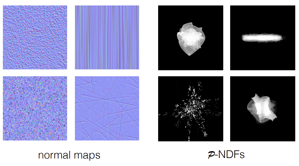
Wave Optics
唯一光源下的金属划痕
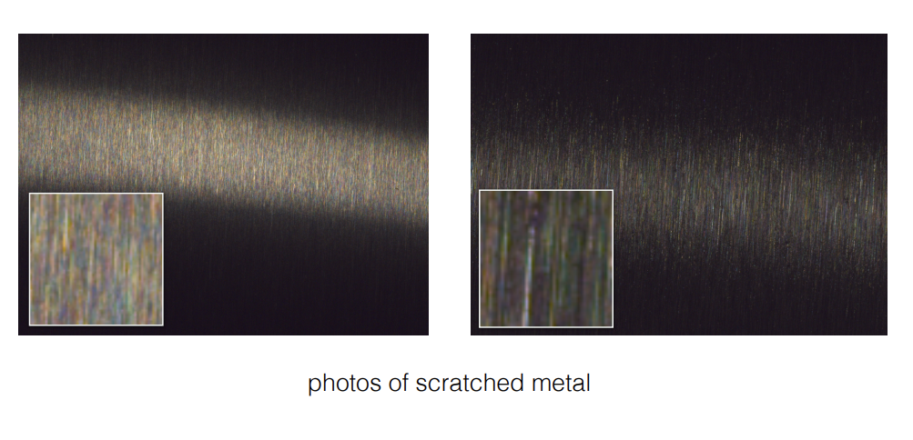
Detailed Material under Wave Optics
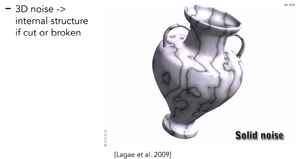
Procedural appearance
-
Define details without textures
-
Compute a noise fuction on the fly
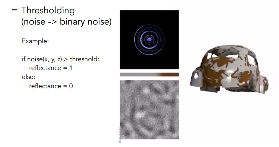
-
-
例如柏林噪波
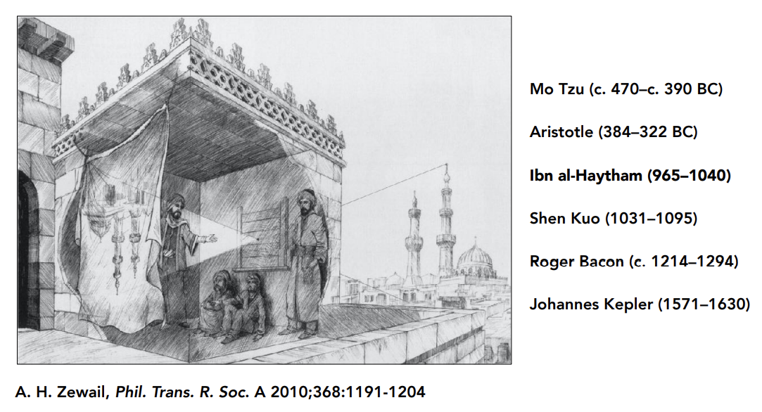
Camera
Imaging = Synthesis + Capture
Inside a camera
-
Phinholes & Lenses For Image on Sensor
-
Shutter Exposes Sensor For Precise Duration
-
Sensor Accumulates Irradiance During Exposure
-
目前传感器只能记录Irradiance,所以需要有针孔或者透镜,来给定记录的方向
-
但是目前有人在研究可以记录radiance的传感器
-
Pinhole Image Formation
注:针孔相机拍不出深度(景深),任何地方都是锐利的,拍不到虚化的存在
光线追踪利用的是针孔相机的模型,也得不出景深效果
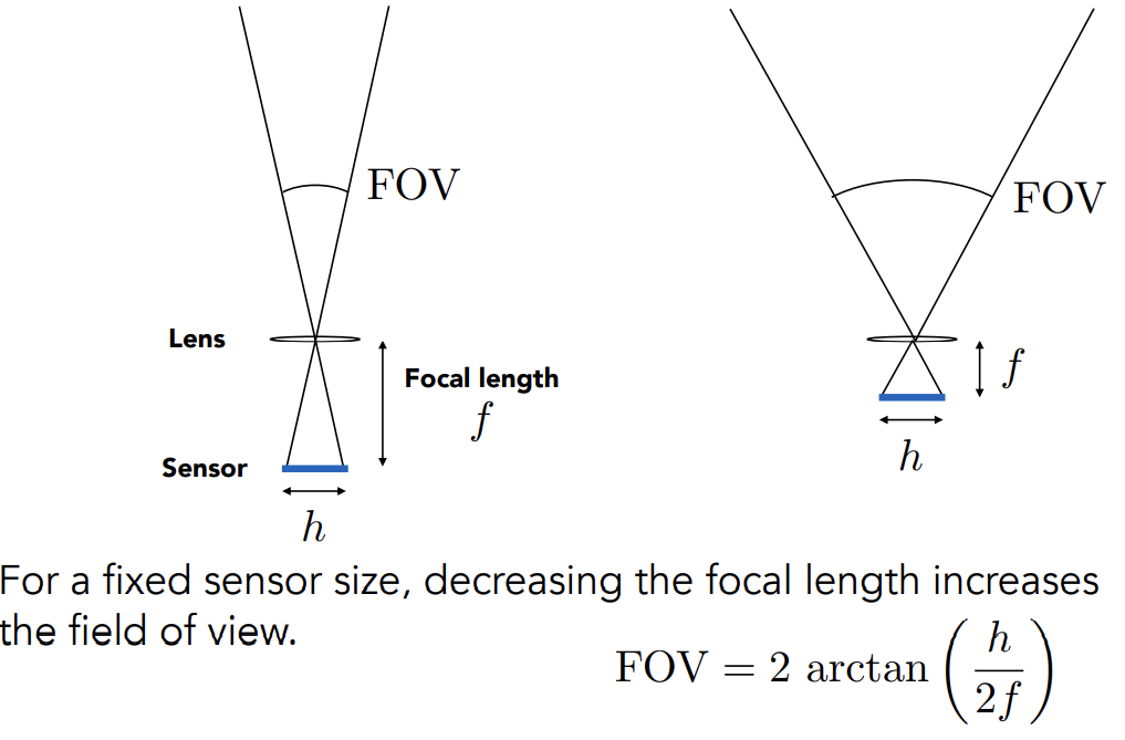
Field of View(FOV)
Effect of Focal Lengh on FOV
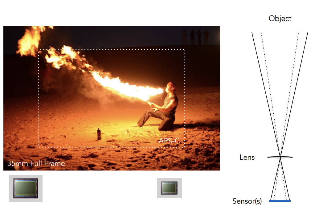
Effect of Sensor Size of FOV
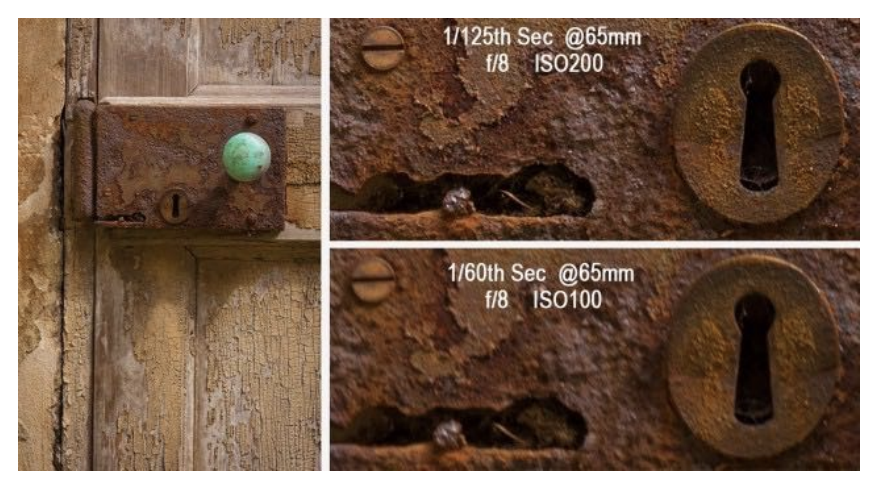
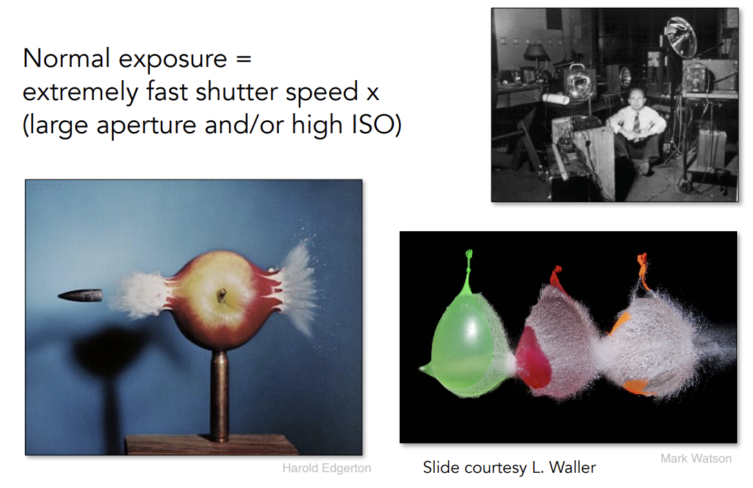
Exposure
H = T x E
-
Exposure = time x irradiance
-
Exposure time (T)
Controlled by shutter
-
Irradiance (E)
Power of light falling on a unit area of sensor
Controlled by lens aperture(光圈) and focal lengh
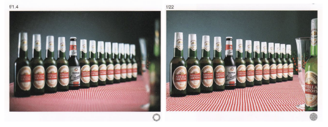
Exposure Controls in Photography
-
Aperture size
Change the f-stop(描述光圈大小的量) by opening / closing the aperture
-
Shutter speed
Change the duration the sensor pixels integrate light
-
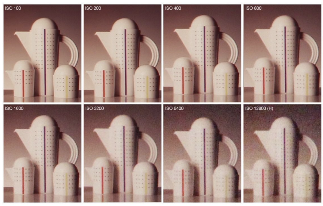
ISO gain(感光度)
Change the amplification (analog and/or digital) between sensor values and digital values
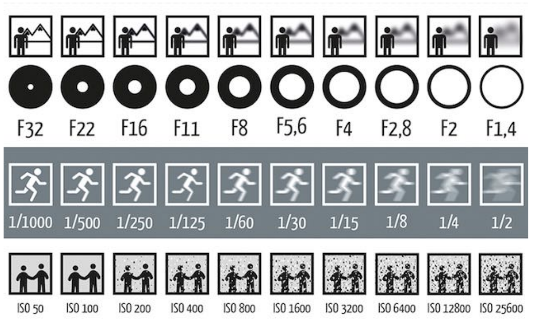
ISO(Gain)
能够提高曝光度,但是同时会放大噪声
F-Number(F-Stop) : Exposure Levels
Written as FN or F/N, N is the f-number
F-Number defined as the focal lengh divided by the diameter of te aperture
可以认为
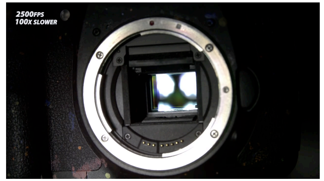
Physical Shutter (1/25 Sec Exposure)
-
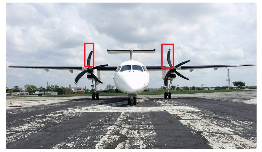
Side Effect of Shutter Speed
-
Motion blur : Handshake, subject movement
-
Boubling shutter times doubles motion blur
-
Rolling shutter : different parts of photo taken at different times
-
High-Speed Photoraphy
-
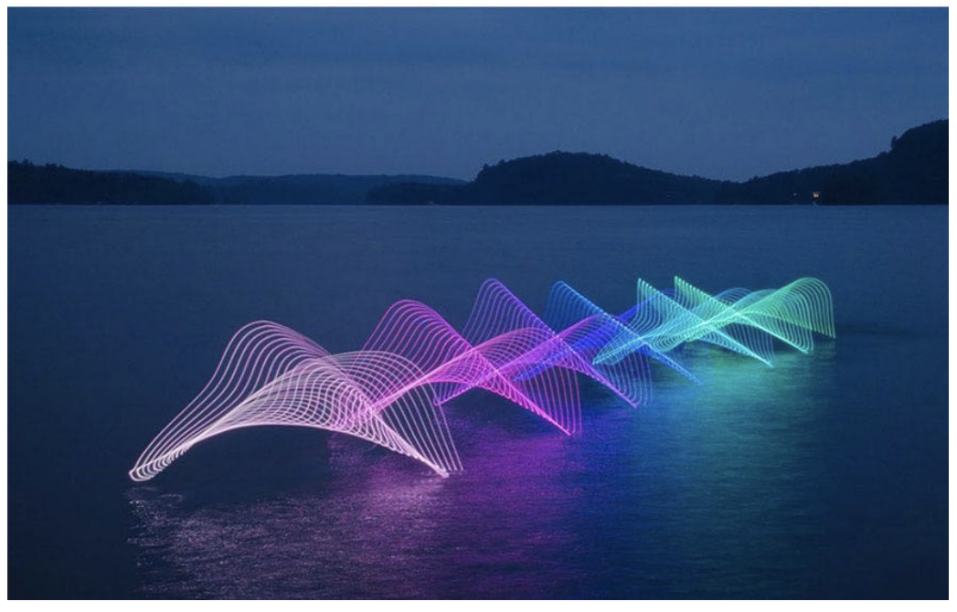
Long-Exposure Photography(延时摄影)
-
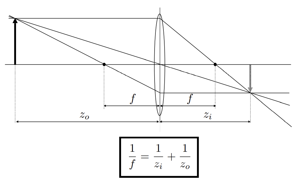
Thin Lens Approximation
The Thin Lens Equation
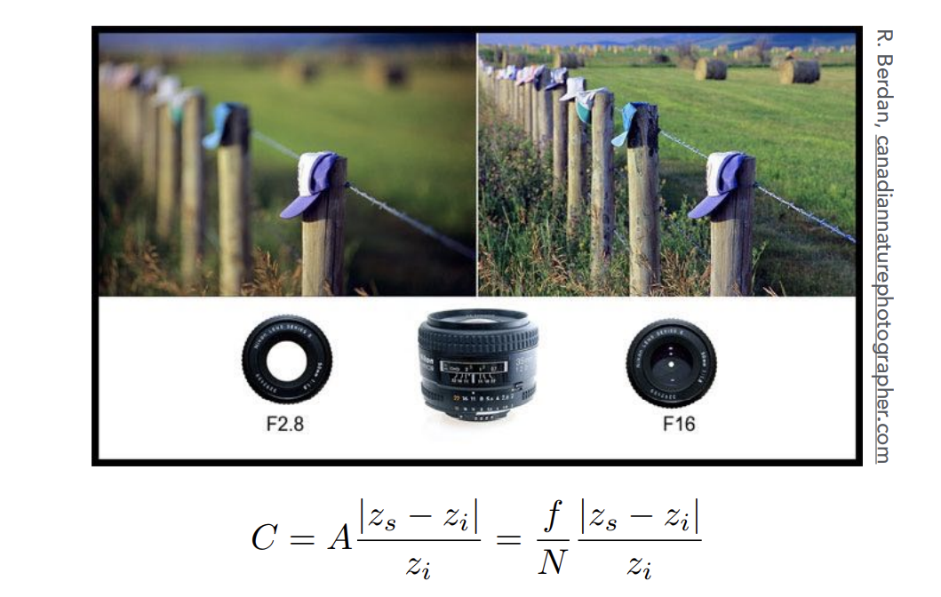
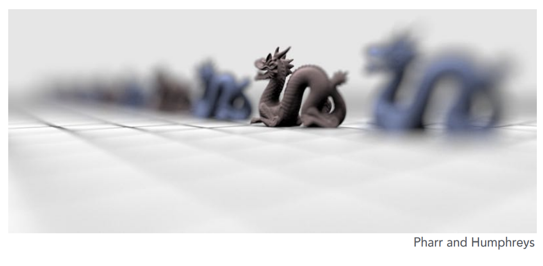
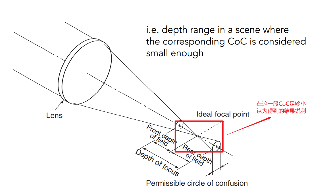
Defocus Blur
-
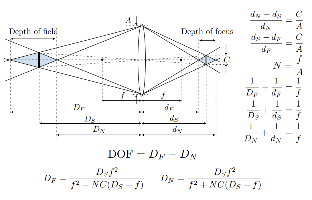
Computing Circle of Confusion(CoC) Size
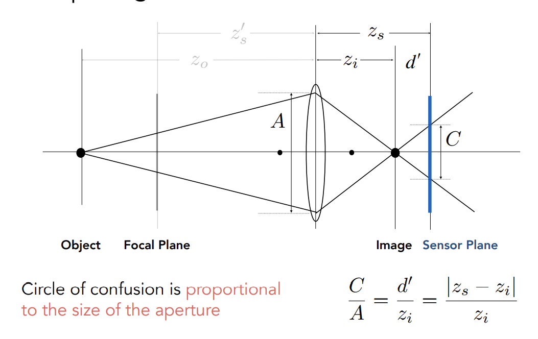
一个点的成像反映到sensor上成了一个圈(近视眼)
-
Circle of Confution取决于光圈的大小
Size of CoC is Inversely Proportional to F-Stop
Ray Tracing Ideal Thin Lenses
原本的Ray Tracing是小孔呈现,但是也可以模拟Lens
Ray Tracing for Defocus Blur (Thin Lens)
Set up:
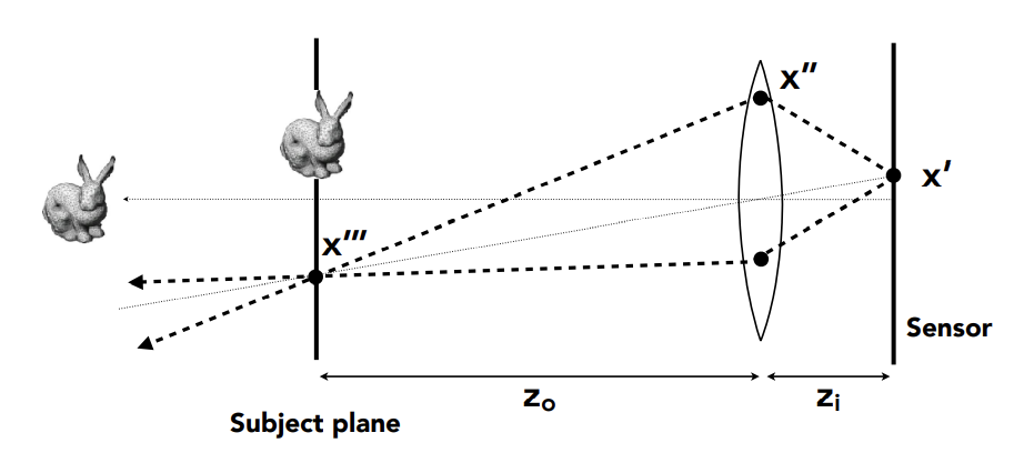
- Choose sensor size, lens focal lengh, and aperture size
- Choose depth of subject of interest (物距)
- Calculate corresponding depth of sensor from thin lens equation
Rendering:
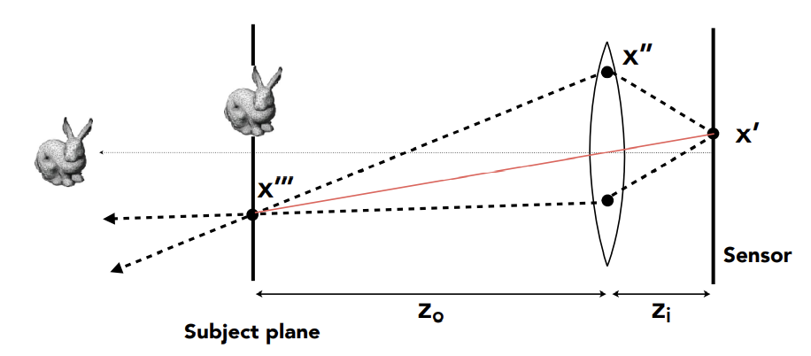
- For each pixel on the sensor
- Sample random points on lens plane
- You know the ray pssing through the lens will hit (using the thin lens formula, because is in focus, consider virtual ray (——center of the l))
- Estimate radiance on ray
Depth of Field
Light Field/Lumigraph
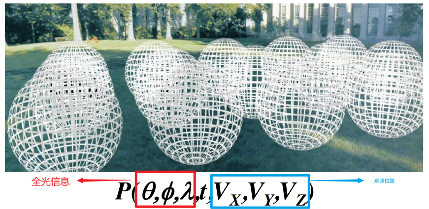
The Plenopic Function
全光函数:Parameterize everything that he can see
is intensity of light
- Seen from a single view point
- At a single time
- Average over the wavelenghs(color) of the visible spectrum
(can also do , but spherical coordinate are nicer)*
Grayscale snapshot
 $$
P(\theta,\phi)
$$
$$
P(\theta,\phi)
$$
Color snapshot
 $$
P(\theta,\phi,\lambda)
$$
$$
P(\theta,\phi,\lambda)
$$
A movie
 $$
P(\theta,\phi,\lambda,t)
$$
$$
P(\theta,\phi,\lambda,t)
$$
Holographic movie
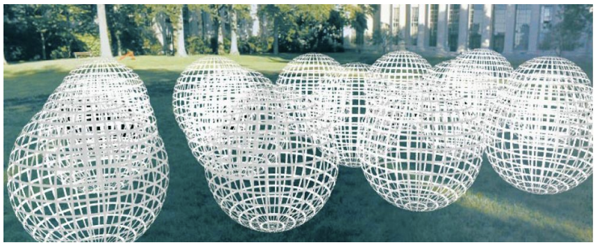 $$
P(\theta,\phi,\lambda,t,V_x,V_y,V_z)
$$
$$
P(\theta,\phi,\lambda,t,V_x,V_y,V_z)
$$
The Plenoptic Function
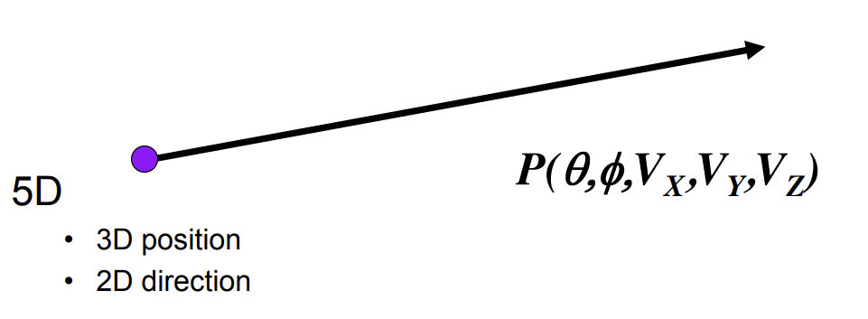
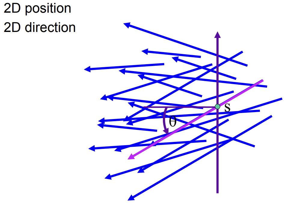
Ray
定义光线:
-
第一类:三维的位置+二维的方向来定义光线
-
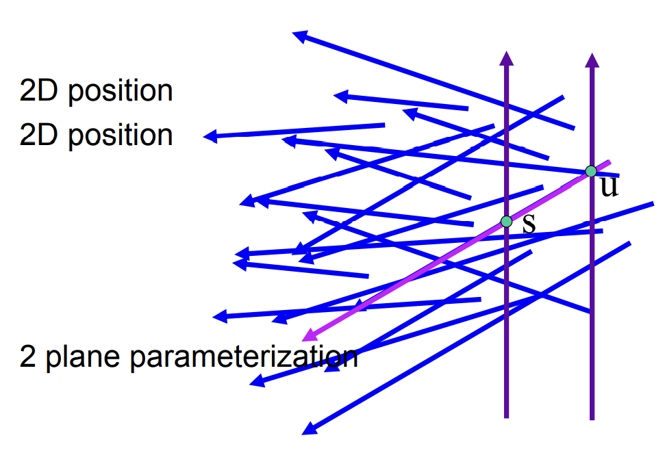
第二类:二维的位置+二维的方向来定义光线
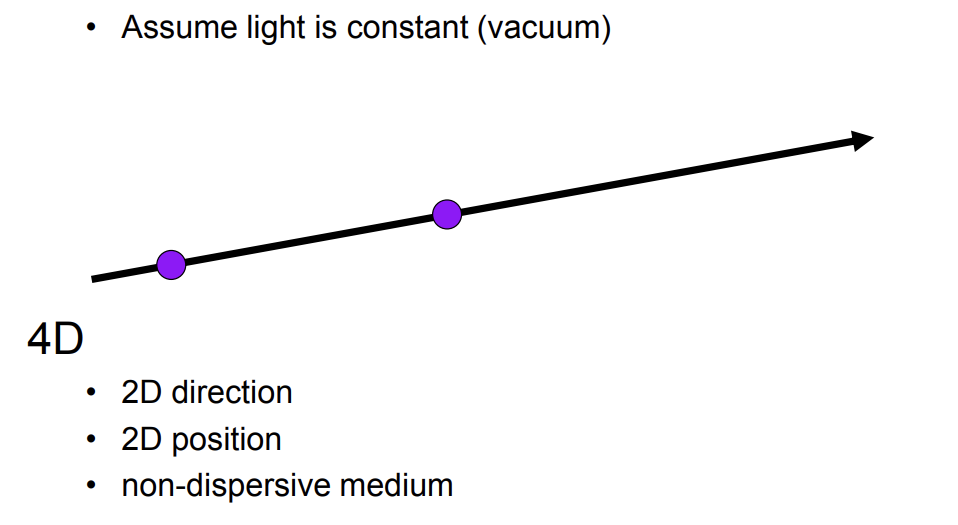
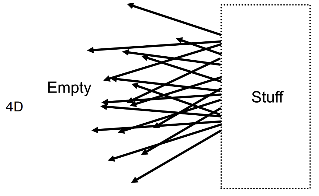
Light Field
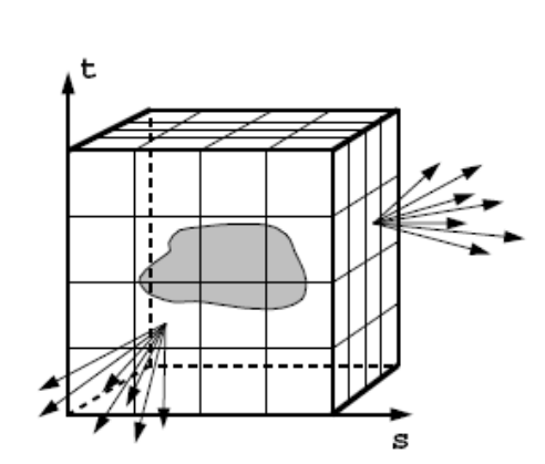
The surface of a cube holds all the radiance information dut to enclosed object
Light Field:函数记录了物体表面不同位置往各个方向的发光情况,光场即为任何一个位置向任何一个方向的发光强度,光场只是全光函数的一部分,只是位置和方向
2D position:只有s和t轴,位置只是在一个面上进行查询,所以是二维的位置
光场的含义:从任意一个位置看向物体,都能查询到各个点的光照信息
记录光场:不需要知道光场内部有什么,只需要查询到储存在表面的任何位置任意方向的光照信息即可
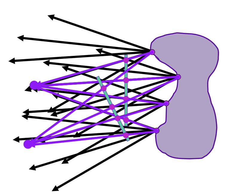
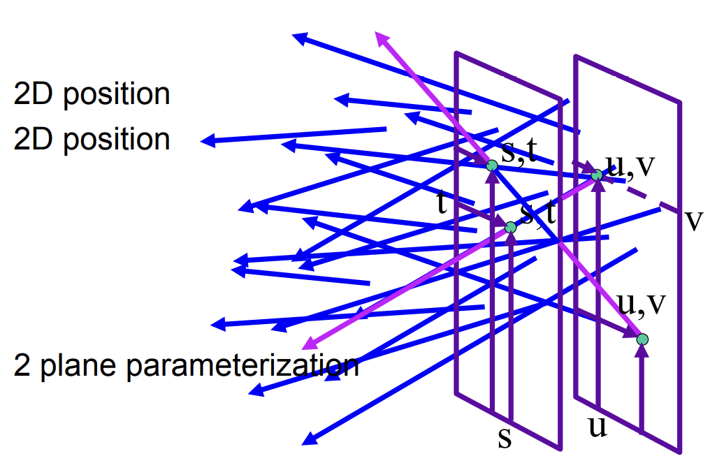
光场的参数化
-
1个位置+1个方向进行参数化
-
两个平行的平面,各自取点进行参数化
-
Lumigraph
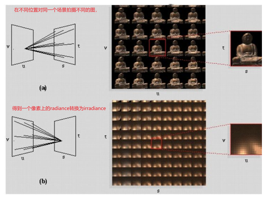
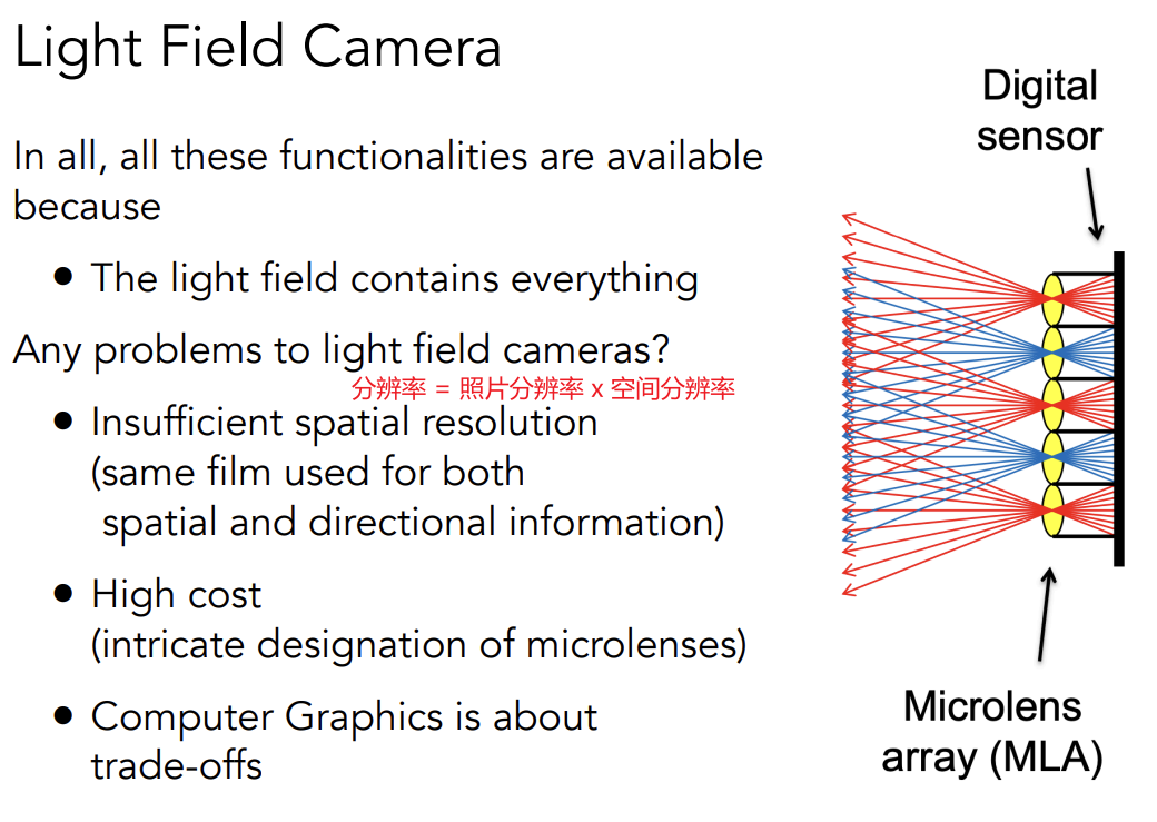
把一个像素分开并在像素前加一个lens,将来自各个方向的光分到不同的位置,即用一个像素储存了不同方向的irradiance
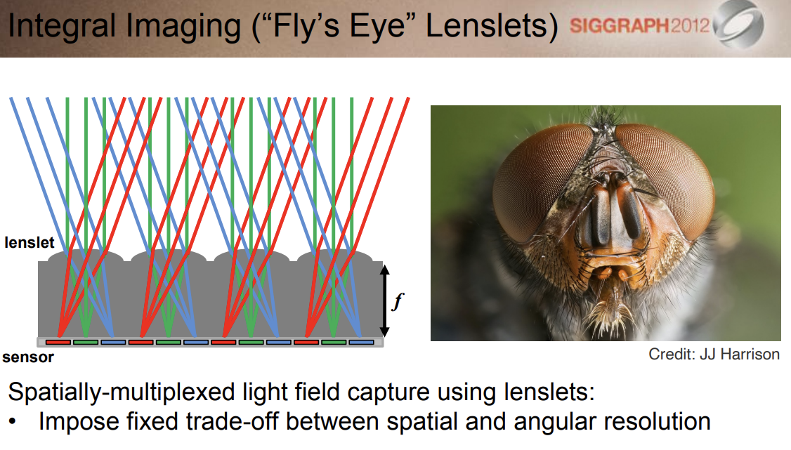
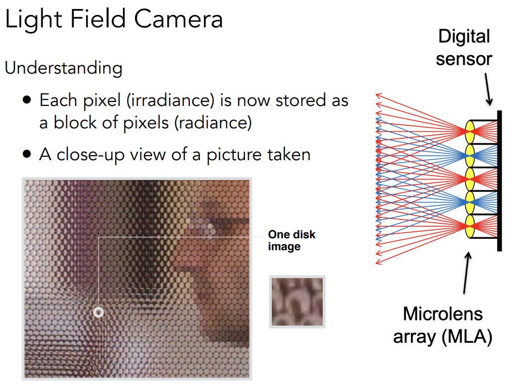
Light Field Camera
原理:微透镜(Microlens),把一个像素替换成一个透镜,使来自不同方向的光通过微透镜分开,分别记录到不同的位置
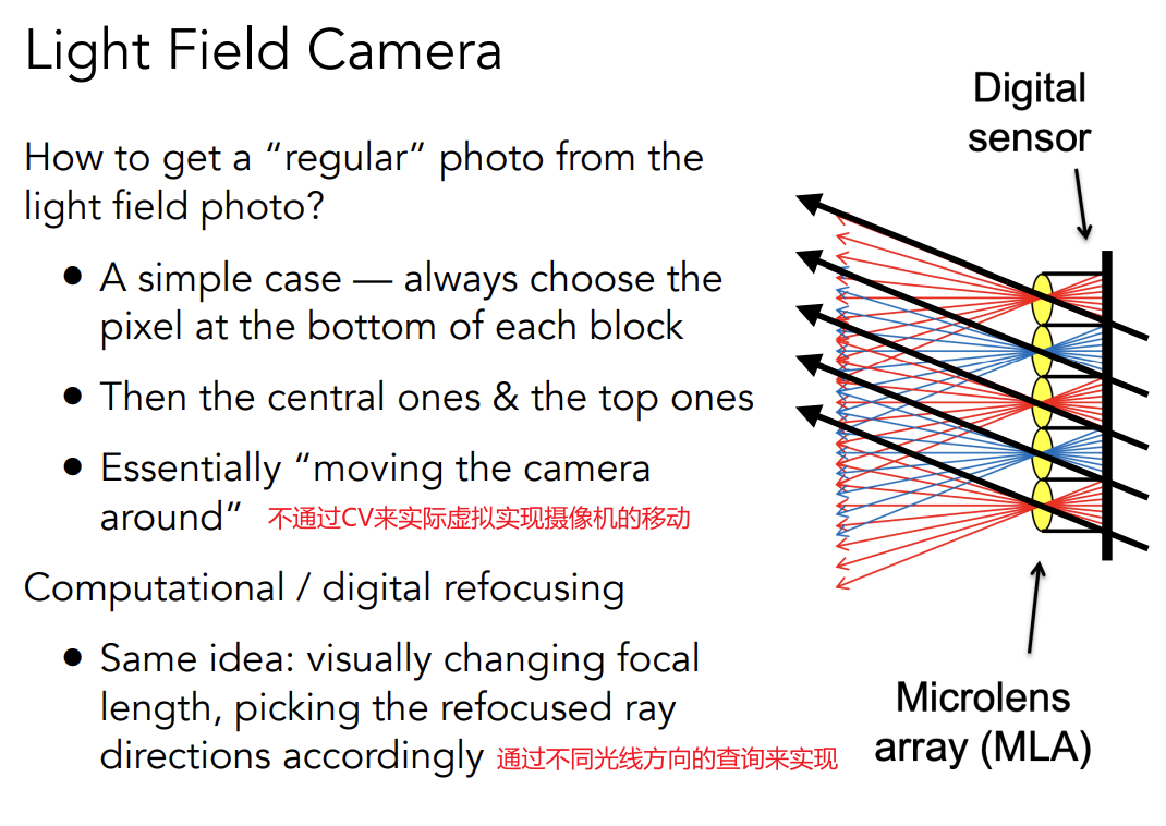
优势:可以后期动态聚焦——先拍照,再聚焦
Understanding
原本像素储存的irradiance被沿着多个方向拆开了(pixelblock of pixels)
Color
Physical Basis of Color
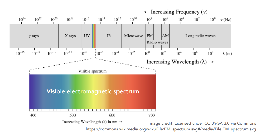
The Visible Spectrum of Light
Electromagnetic radiance
-
Oscillations of different frequencies (wavelenghs)
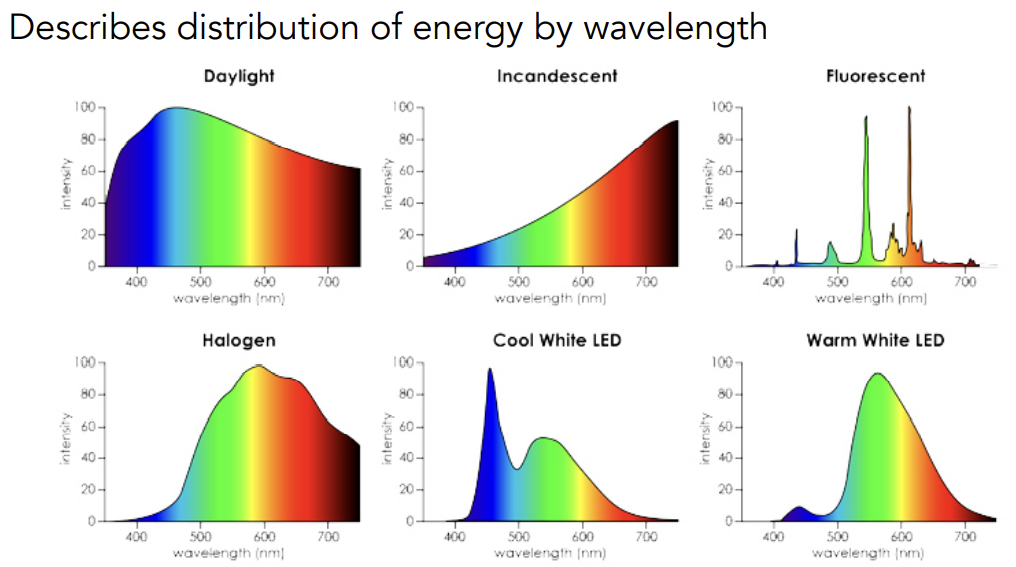
Spectrual Power Distribution (SPD)
Salient property in measuring light
即光线不同的波长对应的强度
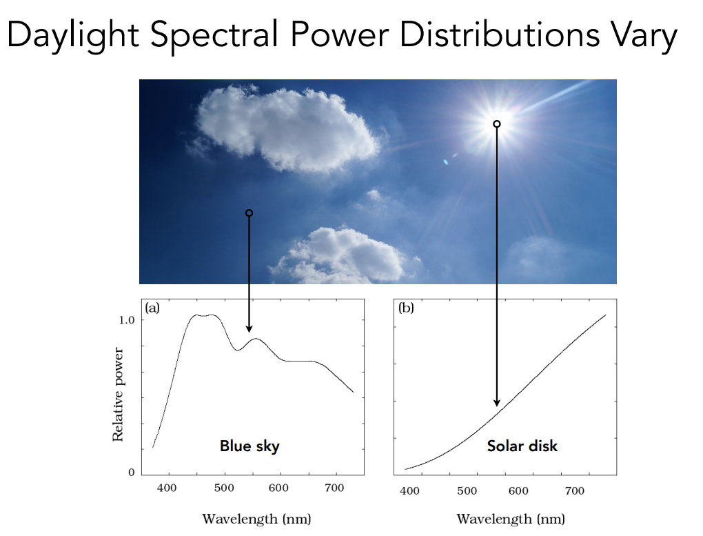
SPD of light sources
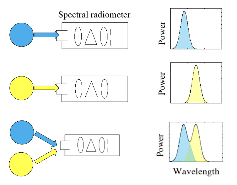
Linearity of SPD:线性关系,可加性
Biological Basis of Color
Anatomy of the Human Eye
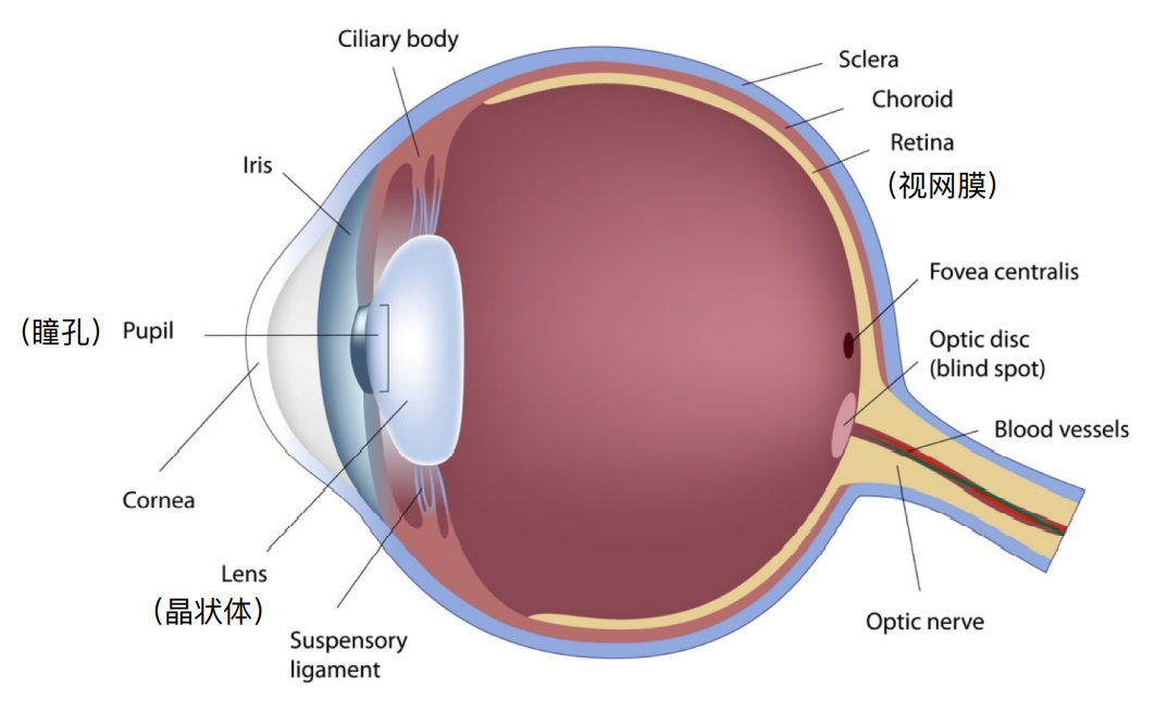
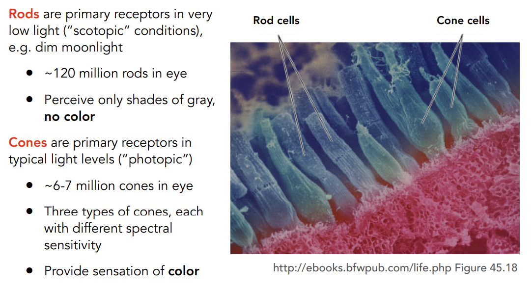
Retinal Photoreceptor Cells:Rods and Cones
-
Rod cells:很多,但是只能感知光的强度,得到灰度图
-
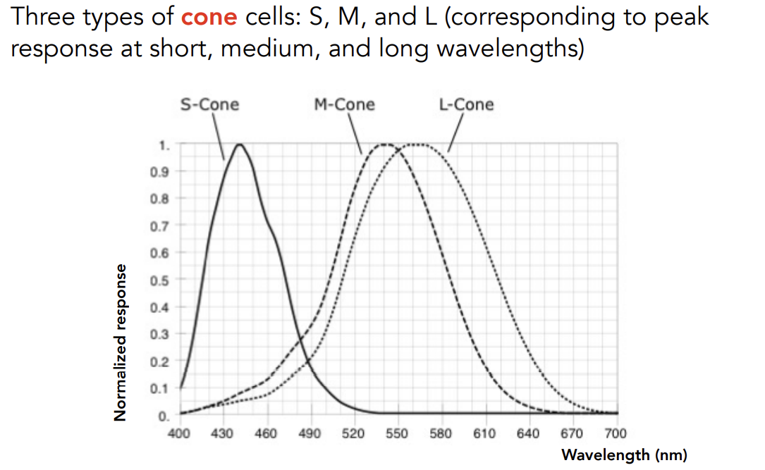
Cone cells:相对较少,能感知光的颜色,又分为三类
- 锥形细胞分类及响应曲线图:
-
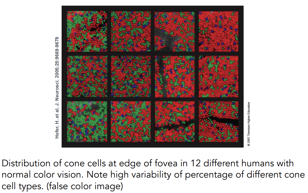
锥形细胞在不同人身上分布的差异很大
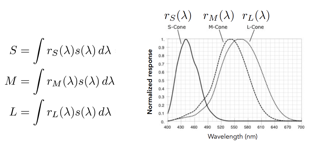
Tristimulus Theory of Color
Spectral Response of Human Cone Cells
感知:光线波长SPD和感知细胞响应曲线相乘的积分,得到的SML才是感知到的颜色,而不是光的SPD
The Human Visual System
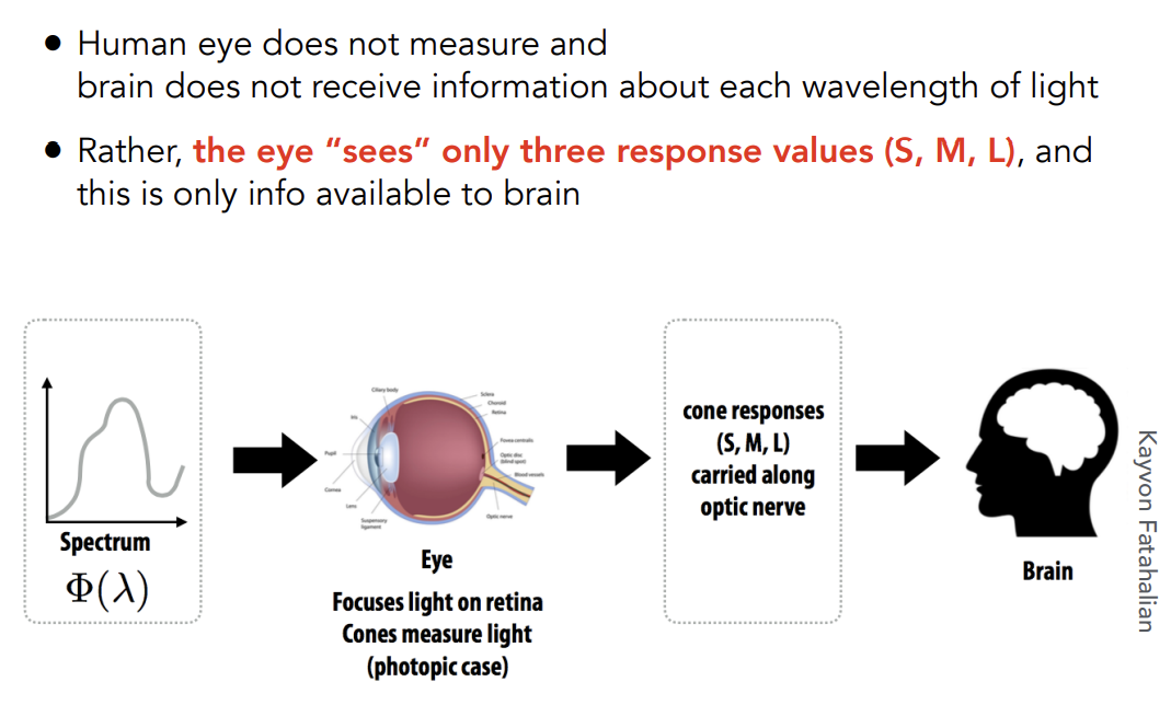
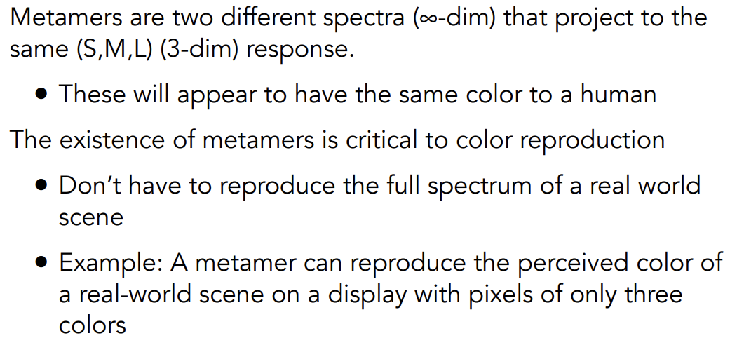
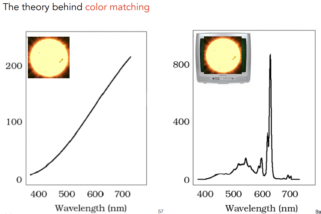
Metamerism
同色异谱现象:不同的SPD但是看到同样的颜色的现象
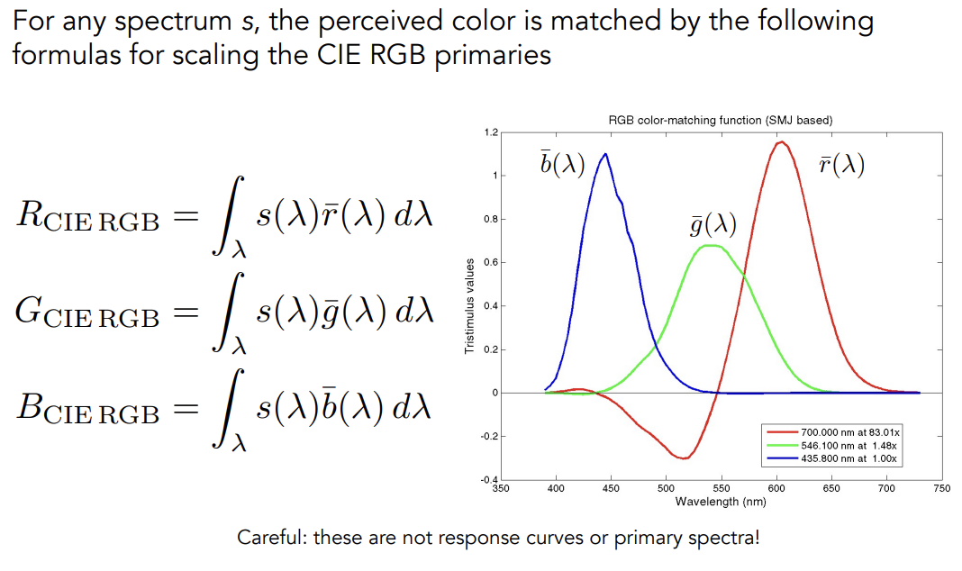
Color matching
Color Reproduction/Matching
Additive Color
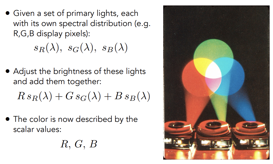
Color Reproduction with Matching Functions
s——SPD
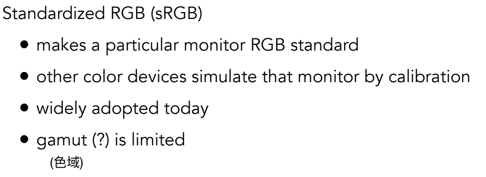
Color Spaces
Standard Color Spaces
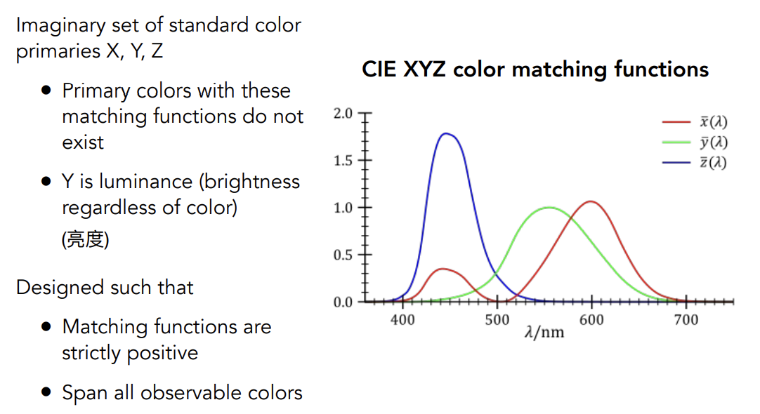
A Universal Color Space: CIE XYZ
另一套匹配系统:一套人造的颜色匹配系统,初值不是存在的颜色
Separating Luminance,Chromaticity
让XYZ系统能表示的颜色显示出来
对大写的XYZ做一个可视化:将XYZ进行归一化(此处的归一和向量不同,此处只是指x+y+z=1),固定了Y,可视化x,y(因为Y只是强度)
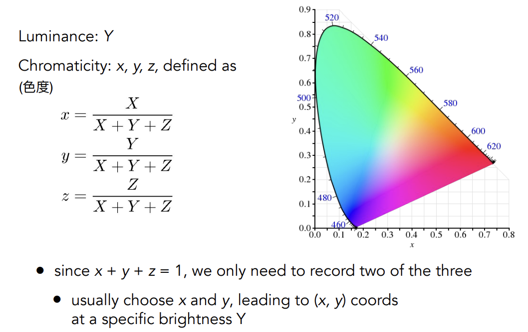
CIE Chromaticity Diagram
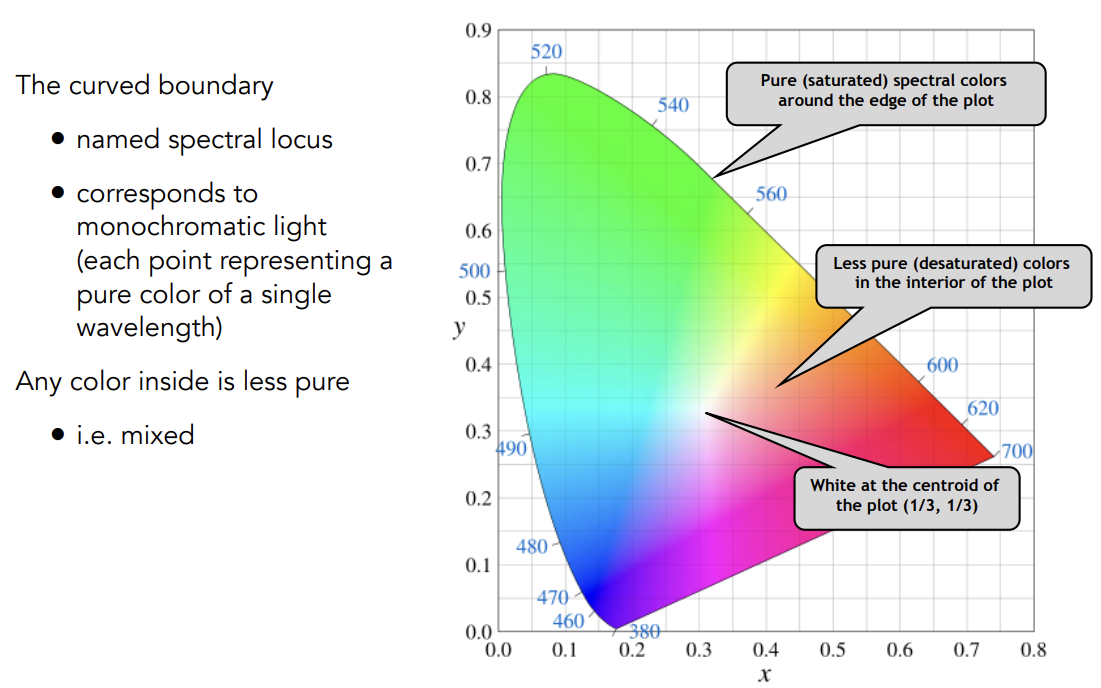
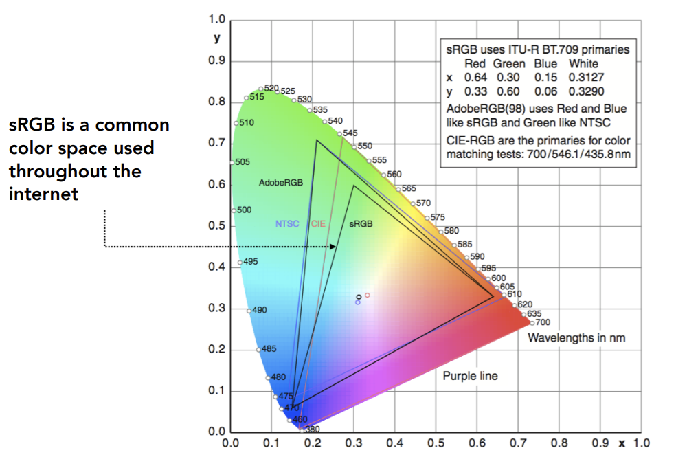
Gamut
不同的颜色空间Gamut色域是不同的
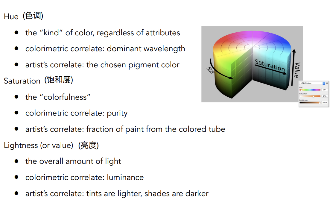
HSV Color Space
Hue—Saturation—Value
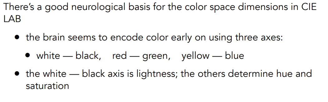
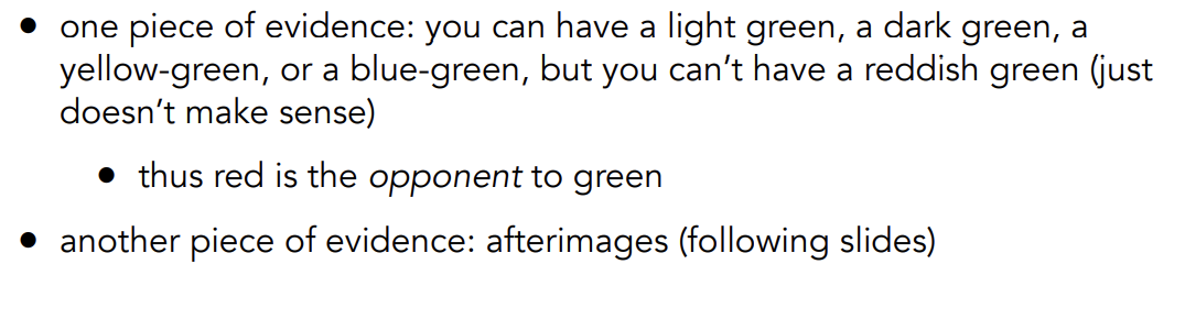
CIELAB Space(AKA L*a*b*)
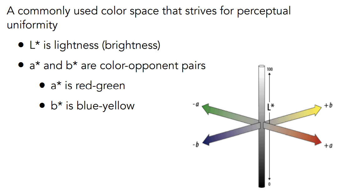
Opponent Color Theory
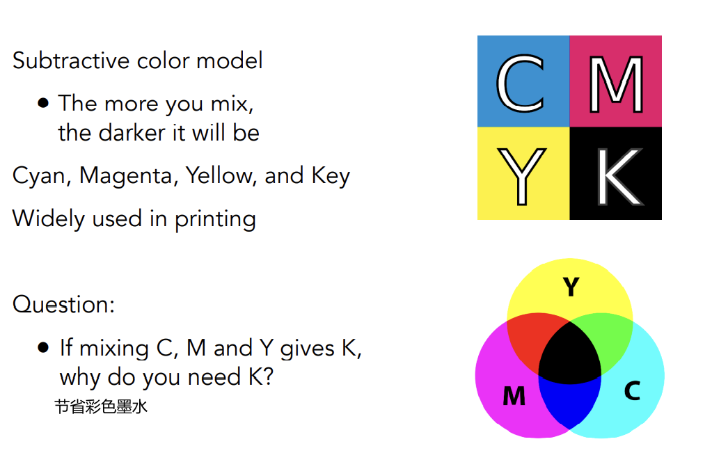
CMYK: A Subtractive Color Space
Animation Intro
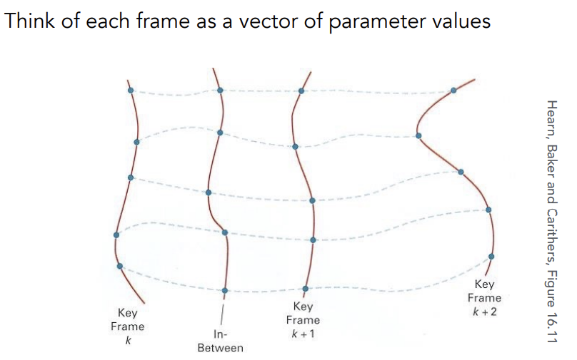
Keyframe Animation
Keyframe
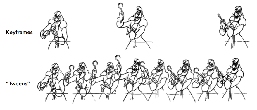
- Lead animator creates keyframes
- Assistant (person or computer) creates in-between frames (“tweening”)
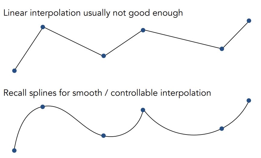
Keyframe Interpolation
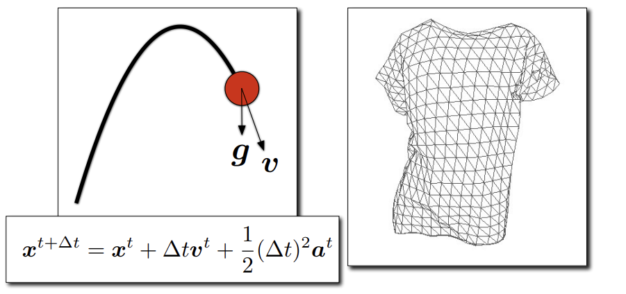
Physical Simulation
- Newton’s Law
-
Generate motion of objects using numerical simulation
-
Example
- Cloth Simulation
- Fluids
- 模拟流体如何运动
- 模拟位置、形状后去渲染,得出模样
- Mass Spring Rope/Mesh(质点弹簧系统)
- Hair
Mass Spring System
A Simple Spring
—— 一系列相互连接的质点和弹簧
Idealized spring
Zero length spring
-
Hooke‘s Law
Problem: this spring wants to have zero length
Non-Zero Length Spring
Spring with non-zero rest length
Problem: oscillates forever
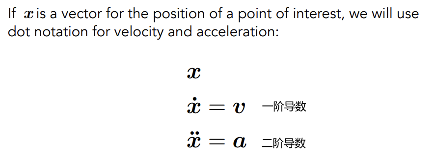
Dot Notation for Derivatives
Internal Damping Force(Energy Loss)
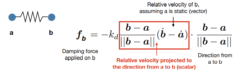
-
is a damping coefficient
-
Viscous drag only on change in spring length
Structures from Springs
-
Behavior is determined by structure linkages
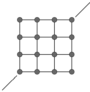
- This Structure will not resist shearing
- This structure will not resist out-of-plane bending (该形状可以折成一个平面并且没有反抗弯曲的力)
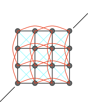
- This structure will resist shearing. Less directional bias.
- This structure will resist out-of-plane bending. Red spring should be much weaker(蓝色线力更强,红色只是用来抵抗弯曲)
Aside: FEM
Finite Element Method(FEM) Instead of Springs
有限元方法,适用于力的扩散与传导
Particle Systems
Particle system
-
Model dynamical systems as collection of large numbers of particles
-
Each particle’s motion is defined by a set of physical (or non-physical) forces (e.g. 粒子之间的碰撞、引力,粒子受到的重力)
-
Popular technique in graphics and games
- Easy to understand , implement
- Scalable: fewer particles for speed, more higher complexity
-
Challenges
- May need many particles (e.g. fluid)
- May need acceleration structure (e.g. to find nearest particles for interactions)
Particle System Animations
For each frame in animation
- [If needed] Create new particles
- Calculate forces on each particle
- Update each particle’s position and velocity
- [If needed] Remove dead particles
- Render particles
Particles System Forces
-
Attraction and repulsion forces
- Gravity, electromagnetism, …
- Springs, propulsion, …
-
Damping forces
- Friction, air drag, viscosity, …
-
Collisions
- Walls, containers, fixed objects, …
- Dynamic objects, character body parts, …
-
Gravitational Attraction
-
Newton’s universal law of gravitation
- Gravitational pull between particles
- Gravitational pull between particles
-
-
Examples
-
Galaxy Simulation
-
Particle-Based Fluids
-
Simulated Flocking as an ODE
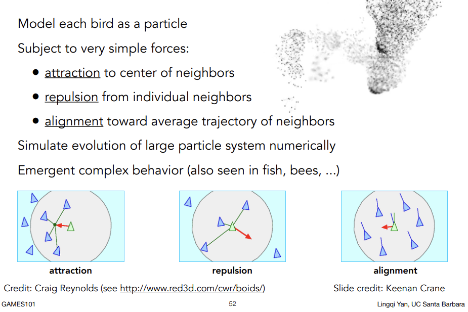
考虑个体与群体之间的联系
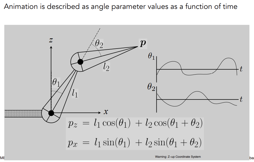
Forward Kinematics
Forward Kinematics
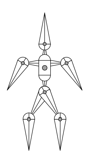
Articulated skeleton
- Topology (what’s connected to what)
- Geometric relations from joints
- Tree structure (in absence of loops)
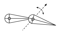
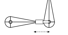
Joint types
-
Pin (1D rotation)
-
Ball (2D rotation)
-
Prismatic joint (translation)
Kinematics Pros and Cons
Strenghs
- Direct control is convenient
- Implementation is straightforward
Weakness
- Animation may be inconsistent with physics
- Time consuming for artists
Inverse Kinematics
Animator provides position of end-effector, and computer must determine joint angles that satisfy constrains
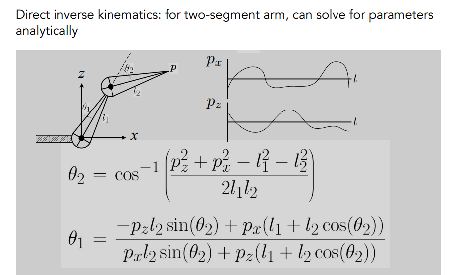
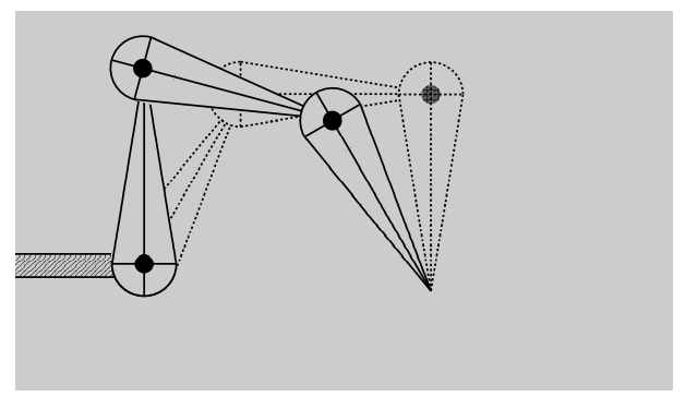
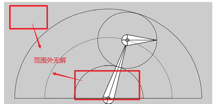
Problems(Hard):
-
Multiple solutions in configuration space
-
Solutions may not always exist
Numerical solution to general N-link IK problem
- Choose an initial configuration
- Define an error metric
- Compute gradient of error as function of configuration
- Apply gradient descent
Rigging
Rigging is a set of higher level controls on a character that allow more rapid & intuitive modification of pose, deformations, expression, etc.
Important
- Like strings on a puppet
- Captures all meaningful character changes
- Varies from character to character
Expensive to create
- Manual effort
- Requires both artistic and technical training
Blend Shapes
Instead of skeleton, interpolate directly between surfaces
Simplest scheme: take linear combination of vertex positions
Spline used to control choice of weight over time
(控制点和控制点之间做插值,blend控制点及控制点周围能够影响的区域)
Motion Capture
Data-driven approach to creating animation sequences
- Record real-world performance
- Extract pose as a function of time from the data collected
Pros and Cons
- Strenghs
- Can acpture arge amounts of real data quickly
- Realism can be high
- Weaknesses
- Complex and costly set-ups
- Captured animation may not meet artistic needs, requiring alterations
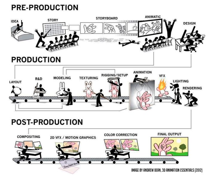
The Production Pipeline
Animation Simulation
Single Particle Simulation
First: study motion of a single particle
Later: generalize to a multitude of particles
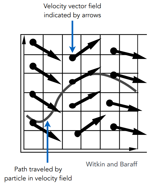
Velocity Field
To start, assume motion of particle determined by a velocity vector field that is a function of position and time:
Ordinary Differential Equation(ODE)
Computing position of particle over time requires solving a first-order ordinary differential equation:
- “first-order”: the first derivative being taken
- “Ordinary”: no partial derivative (i.e. x is just a function of t)
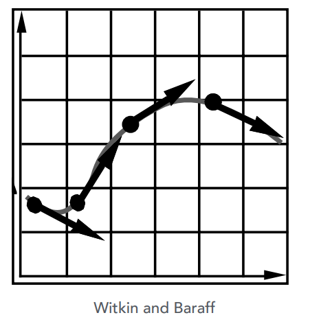
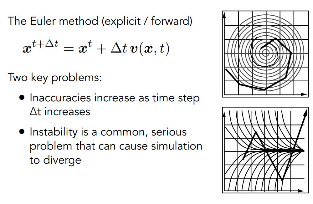
Euler’s Method
-
Simple iterative method
-
Euler’s Method - Errors
With numerical integration, errors accumulate
增大time step可以减小误差
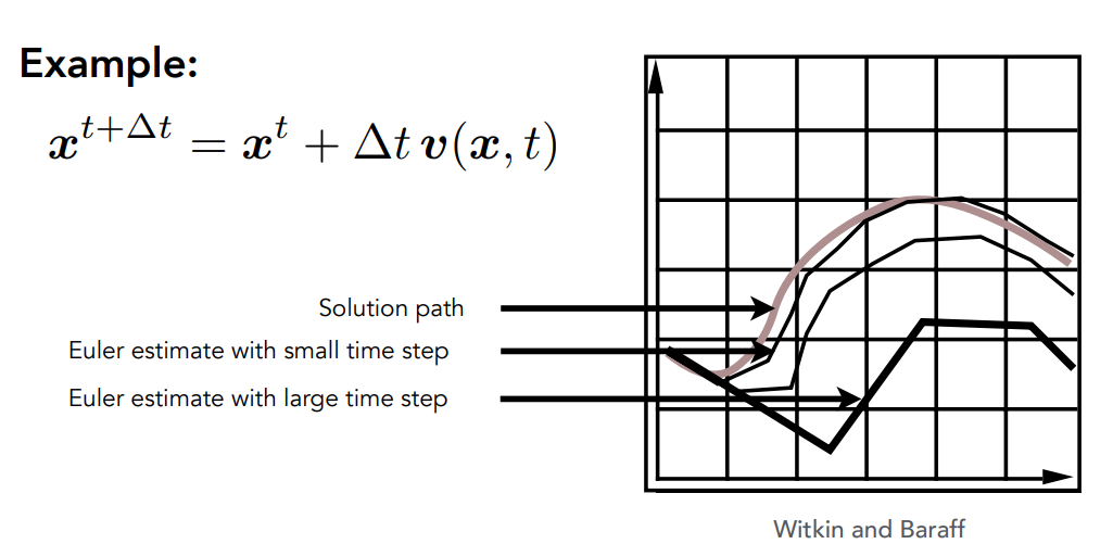
time step affect the accuracy
-
Instability of Euler Method
不稳定,例如要沿着下面的圆形移动,但不管time step有多小,往下进行会越来越脱离想要的结果
Errors and Instability
Solving by numerical integration with finite differences leads to two problems:
-
Errors
-
Errors at each time step accumulate
Accuracy decreases as simulation proceeds
-
Accuracy may not be critical in graphics applications
-
-
Instability
- Errors can compound, causing the simulation to diverge even when the underlying system does not
- Lack ok stability is a fundamental problem in simulation, and cannot be ignored
Combating Instability
How to determine/quantize “stability”?
-
Local truncation error(every step) / total accumulated error(overall)
-
这些数字没有意义,研究的是他们的导数
-
Implicit Euler has order 1, which means that
-
Local truncation error:
-
Global truncation error:
(h is the step, i.e. )
-
-
Understanding of
If we halve h, we can expect the error to halve as well
Midpoint Method/Modified Euler
- Average velocities at start and endpoint
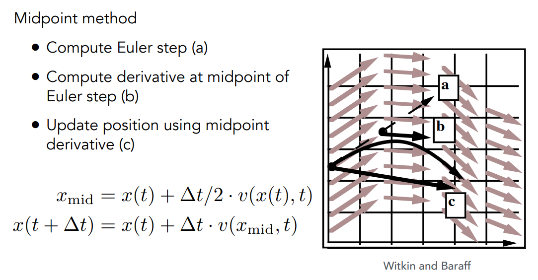
理想运动路径是中间的曲线,实际路径是下面的直线
实际上是用了两次Euler方法,先用出发点的速度场来算出中点b的速度,在以此速度回到起始点作为真正的速度
-
Better results: 算出的局部的二次模型,优于原本的一次模型
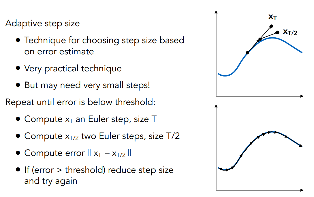
Adaptive Step Size
试着把分成两个部分,如果两个结果相差很远,就减小step size并再次进行判断
得到右下的图,在不同的位置会有不同的
Implicit(Backward) Euler Method
-
Use derivatives in the future, for the current step
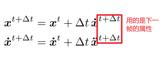
-
Solve nonlinear problem for and
-
Using root-finding algorithm
-
Offers much better stability
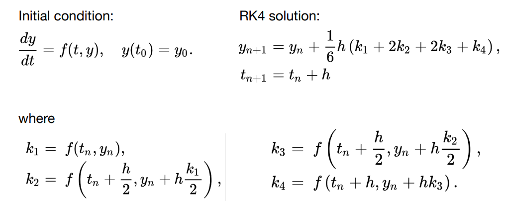
Rung-Kutta Families
A family of advanced methods for solving ODEs
- Especially good at dealing with non0linearity
- It’s order-four version is the most widely used
Position-Based/Verlet Integration
-
Idea:
- After modified Euler forward-step, constrain position of particles to prevent divergent, unstable behavior
- Use constrained positions to calculate velocity
- Both of these ideas will dissipate energy, stabilize
-
Pros and cons
- Fast and simple
- Not physically based, dissipates energy(error)
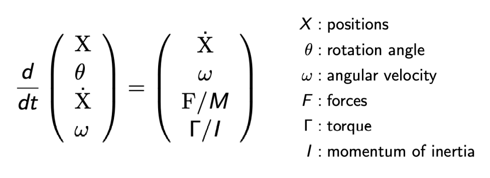
Rigid Body Simulation
物体内的所有点运动规律都一致
Simple case
- Similar to simulation a particle
- Just consider a bit more properties
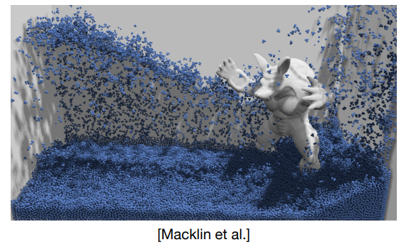
Fluid Simulation
A Simple Position-Based Method
Key idea
- Assuming water is composed of small rigid-body spheres
- Assuming the water cannot be compressed(i.e. const density)
- So, as long as the density changes somewhere, it should be “corrected” via changing the position of particles
- You need to know the gradient of the density anywhere w.r.t. each particle’s position
- 任何一个位置上让原本不正确的密度恢复原本的密度,并且我知道如何调整各个小球的位置使得他的密度往我们所需的方向上去变化——Gradient Descent
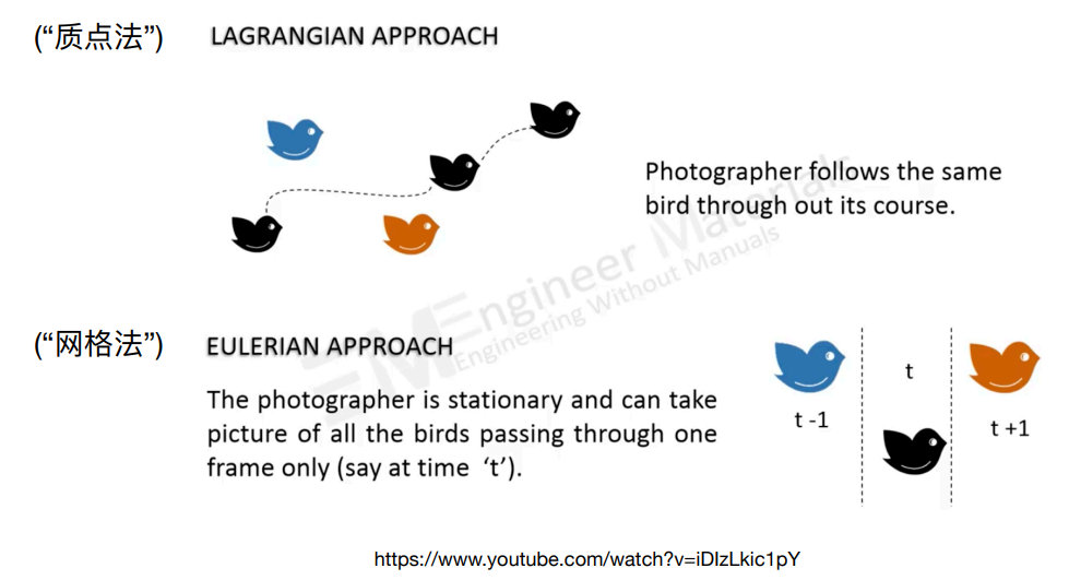
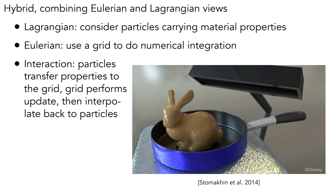
Eulerian vs. Lagrangian
Two different views to simulating large collections of matters
Material Point Method(MPM)
—Next—
- Games201 —— Advanced Physics Engines 2020: A Hands-on Tutorial
- Real-Time High Quality Rendering